A retired golf pro has teamed up with a land development company to build a world-class resort that includes three golf courses, lodging, restaurants, and other amenities. The resort will be located in the pro's home state of Oregon. An earlier analysis identified three counties in which to locate the resort. The two more rural counties—Jefferson and Crook—were favored by the pro, while the development company preferred Deschutes County, which includes the region's largest city.
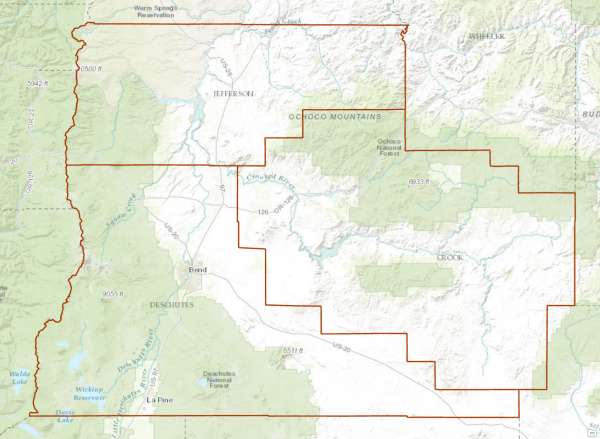
Read about the development company's initial analysis.
Since then, the project has been on hold. Several of the investors the company had lined up for the project are expressing concerns about the pro's commitment to the project given his other obligations and his rumored mercurial nature. After numerous meetings and phone calls to reassure the nervous investors, the company is ready to restart the project and move to the next phase—looking for specific locations to build the resort.
A vision
The pro has a vision for the resort's setting: nestled among forest and meadows, but also including grasslands and scrub to give the hikers and equestrians a taste of the Wild West. In his mind's eye he also sees a nearby flowing river, and of course spectacular views of surrounding mountain peaks. The pro wants the resort to have the feel of a retreat, so visitors get a sense that they are away from civilization. That's all fine, the development company management agrees, but they argue that accessibility is the real key to success. This part of the state is already somewhat remote; they surmise that the upscale clientele they hope to attract are more likely to fly in on commercial flights or private planes than to drive, so they want to ensure that the resort is a short drive from an airport.
The pro originally told the developers that the resort would require 500 acres, based on his past experience developing single golf courses, which cover about 100 acres. However, he now tells them that he recently had an informal discussion with his favored golf course architect. In the architect's opinion, while a 500-acre site would likely accommodate three courses, it would be a tight fit and would leave little space for all the other amenities the pro envisions: equestrian and hiking trails, stables, lodging, and restaurants, not to mention space for all the service functions required to support these facilities.
The architect—not one to mince words—told the pro that unless he wants his fairways to double as equestrian paths he'll need at least twice—and probably three times—as much land to create the ambience he wants for his resort, up to 1,500 acres.
The developers are a bit taken aback at this news—the land costs for the project have tripled overnight. Still, the developers are confident there is enough private land available that they will be able to put together the parcels needed for the larger resort. And while their current investors are likely to balk at putting up any more funds, they are pretty sure they can bring in a few more investors if needed. The pro also agrees to increase his investment—it's been a good couple of years for him. He's been doing guest appearances on golf television shows, which has increased his visibility and led to some lucrative licensing deals for equipment and sportswear. The developers decide to move ahead with the site selection phase. To keep their options open, the initial phase of the analysis will include all three counties.
Turning the vision into reality
The GIS team in the development company's acquisitions division picks up the analysis project. The goal is to identify at least five suitable locations for the resort. The first task is to convert the pro's vision of the setting for the resort, and the company's requirements for access, into criteria that specify what makes a location suitable.
The analysts quickly identify the criteria—surrounded by a variety of landscape types, near a river, near an airport, and with a view of mountain peaks. They know that any suitable locations will need to be on relatively gentle slopes to accommodate the golf courses themselves. And, of course, they will incorporate the earlier layer of privately owned land they created to ensure the suitable sites are potentially available for purchase and development. They now know the data layers they will need for the analysis.
| Criterion | Data layer |
|---|---|
Near a variety of landscape types | Land cover |
Near a river | Major rivers |
Near an airport | Public airports |
View of mountain peaks | Peaks/Viewshed (Elevation) |
Gentle slopes | Slope (Elevation) |
Private land ownership | Land ownership |
Before going any farther, the analysts give some thought to the analysis method they will use. For the earlier analysis, which involved a simple polygon overlay, they employed ArcGIS Online. The current analysis will be more involved. They note that several of the layers they need for the analysis will originate as raster layers. Creating both the slope and viewshed layers will require a raster elevation layer, and the land-cover data they have in mind—from the National Land Cover Database (NLCD)—is also stored as a raster. They decide raster overlay analysis is the way to go. Using rasters will also allow them to easily assign weights to each of the layers so they can, for example, give a higher priority to gentle slopes than to mountain views.
To perform the raster analysis, they will need to switch from ArcGIS Online to ArcGIS Desktop and use either ArcMap or ArcGIS Pro.
As it turns out, the team leader recently returned from the Esri User Conference, where she learned about a new tool in ArcGIS Pro called Locate Regions. This tool takes a raster suitability surface as input and identifies the best areas, or regions, of a given size and shape. It sounds like exactly what they need to do. They've created suitability surfaces for previous projects—this new tool will allow them to take the analysis to the next step and identify the best specific locations for the resort. So ArcGIS Pro it is.
The immediate task is to create a suitability surface. Once that's complete they can run Locate Regions to identify the suitable sites for the resort. From their past experience they know that creating the suitability surface is a multistep process: collecting the source data layers, performing any required processing to create the criteria layers, reclassifying the criteria layers using a common scale, and finally combining the reclassified criteria layers to create the suitability surface.
They set about collecting the source data layers. The land ownership layer they already have from the earlier analysis. They get land cover and major rivers from the statewide GIS data clearinghouse. They need an elevation surface to create the slope layer as well as the layer of views of peaks (which, of course, also requires the layer of mountain peaks). They find these, as well as a layer of both commercial and general aviation airports, online in the Living Atlas.
In reviewing the data layers they've collected, they quickly discover an issue they'll need to consider. While the analysis focuses on the land within the borders of the three counties, for several of the criteria, they will want to include features outside the borders to make sure the criteria layers accurately reflect reality. The nearest airport to a potential site may be in an adjacent county. Similarly, a river that can be seen from a potential site might be just outside the border of the county. And they will definitely want to include distant mountain peaks that can be seen from within the counties. When creating the criteria layers, they'll want to include any of these features that are outside the county borders. But how far outside? They see they'll need to start making some decisions on the criteria values—at least the maximum value they want to consider for these criteria.
For rivers, they conclude that any rivers more than a mile or two from a site are not going to enhance the visual quality or experience of the site. For mountain peaks, based on the visibility of major peaks from cities in the region, they decide that any peaks more than 40 miles from a location are not likely to add much in the way of views. As for distance from airports, after a discussion with the company's marketing team, they decide that they will limit the airports to be included to those within 50 miles of the county borders. Any airports farther than this are unlikely to be used as destinations for accessing the future resort. For now, this will give them limits they can use to create the criteria layers.
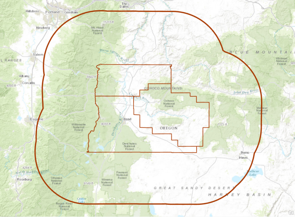
Some of the source layers cover the entire state, and some cover the entire country or continent. To ensure the criteria layers all cover the same area—the three counties and vicinity—they decide to create a buffer of 50 miles around the counties and use this layer to define the extent as they create the criteria layers. This will also speed up the processing. Using the 50-mile buffer will ensure that any features they need that are outside the county borders (peaks, rivers, or airports) are included.
Creating the criteria layers
With the source data layers in place and the parameters for the criteria layers specified, the analysts set about creating the layers. Each will require its own set of steps.
Land ownership
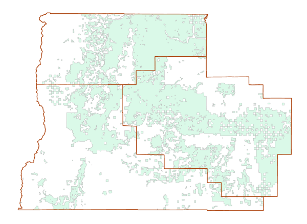
The layer of private land ownership, created during the initial study, is a feature layer of polygons. Since any potential locations for the resort have to be on private land, the analysts decide to use this layer as a screen, or mask, when they create the suitability surface. Any otherwise suitable cells that occur outside the private land will be off limits (in raster lingo, they will be assigned a value of NoData) and will not be included when Locate Regions is run. No additional processing is needed for this layer.
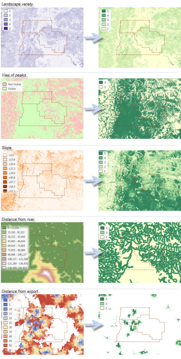
Landscape variety
The goal for this layer is to represent the variety of landscape types surrounding any given cell. Currently the land-cover layer has sixteen different types, plus a category for any cells that are unclassified.
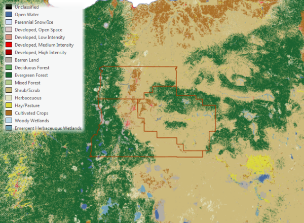
Reasoning that most visitors to the resort will not distinguish between, for example, three different types of forest or two different types of wetlands (with the exception of the occasional golfing ecologist), the analysts decide to generalize the layer into fewer, broader categories. Since the goal of including this layer is to find locations that have a variety of aesthetically pleasing landscapes, they exclude any developed areas and barren land, as well as perennial snow and ice (knowing that the resort is not going to be located on a mountain top). The result is a layer with five values (the values of 1 through 5 are numeric codes used to identify each category).
| Land-cover type | Reclassify value |
|---|---|
Open Water | 1 |
Deciduous Forest | 2 |
Evergreen Forest | 2 |
Mixed Forest | 2 |
Shrub/Scrub | 3 |
Herbaceous | 3 |
Hay/Pasture | 4 |
Cultivated Crops | 4 |
Woody Wetlands | 5 |
Emergent Herbaceous Wetlands | 5 |
All Other Categories | NoData |
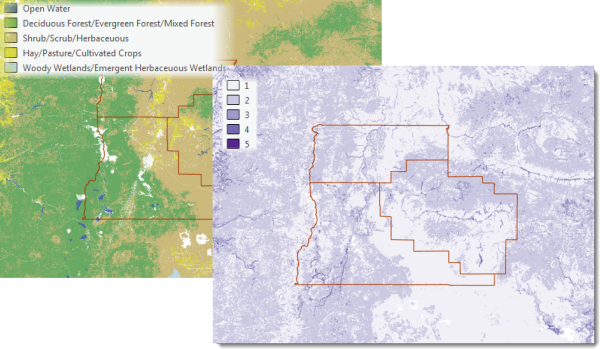
Next they run the Focal Statistics tool, specifying Variety as the statistic to calculate. Figuring that most visitors to the resort will experience their surroundings on foot or horseback, they set an analysis window of about a quarter mile (1,200 feet, to be exact). Visitors are not likely to be aware of areas farther than that distance from any given point. For each cell, the tool calculates the number of different landscape types in a quarter-mile-square area around that cell. As it turns out, the number of types ranges from a minimum of one to a maximum of five, so the map has values of 1 through 5.
Distance from rivers
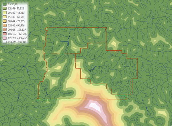
The processing for this layer is pretty straightforward. First, the analysts select rivers within a mile of the county borders (in case the nearest river to a location is just outside the county). Then they run the Euclidean Distance tool to create the distance surface.
Slope
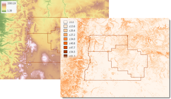
Creating the slope layer is even simpler. The analysts run the Slope tool, using the elevation layer as input.
Distance from airports
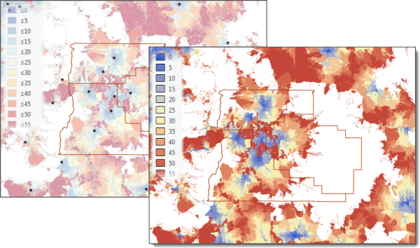
To better model reality, the analysts want to specify the distance from airports using driving time in minutes, rather than distance in miles. One team member suggests that they could simply calculate Euclidean distance from airports and estimate the drive time from the distance in miles. But this approach assumes travel is in a straight line, not over the road network. One of the other analysts thinks they might be able to create a cost-distance surface, assigning cells with roads a lower cost to approximate travel over roads. They all agree that distance from airports is an important criterion, so they want to be as accurate as possible. In the end, they decide to create drive-time areas, specifying 5-minute increments. They then convert this layer to a raster layer. The resulting layer shows how far each cell is from a public airport (within a 5-minute window), taking into account travel over highways and local roads. Earlier, they had used a 50-mile cutoff to identify airports to include in the analysis. Now, after checking again with the marketing analysts, they limit the drive time to a maximum of 60 minutes. Any locations more than an hour's drive from an airport will be off limits.
View of mountain peaks
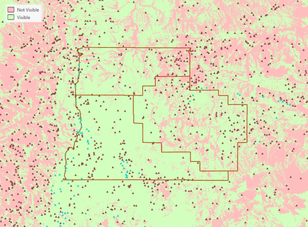
Realizing that some peaks are more impressive than others, the analysts decide to include only those that are over 2,000 meters in elevation (lower peaks will not provide the dramatic views the golf pro envisions). Of these, they select the ones within 40 miles of the county borders and then run the Viewshed tool, using the selected peaks and the elevation layer as inputs.
Creating the suitability surface
The analysts now have the criteria layers. To create the suitability surface, they'll add them together. However, as the analysts are well aware, the layers all have different measurement units. While the value of a cell in the distance from rivers layer is measured in miles, the value of that cell in the distance from airports layer is measured in minutes. Slope is measured in degrees, the viewshed layer measures the number of peaks visible from each cell, and the landscape variety layer measures the number of different landscape types surrounding a cell. Clearly these values can't be added together and produce a meaningful result.
The analysts need to perform one more step for each layer before adding the layers together. They'll reclassify each of the layers using a common scale, assigning the existing values to levels ranging from most suitable to least suitable. Since the layers will be added, they'll assign a high number to most suitable and a low number to least suitable, so that in the final suitability surface the highest number will represent the highest suitability.
The analysts meet to decide how many levels the scale needs to have. They start by discussing how they might slice up the values for each of the individual criteria layers. For distance to rivers, for example, they decide that if a cell is more than a couple of miles from a river, it would get a low suitability rating. The river is too far away, in those cases, to add much aesthetic value to the location. Cells within a mile would get a high rating—the river might run through the resort or would at least be close enough to ride or walk to. Cells between one and two miles from a river get a rating in the middle. So for rivers, they really only need three levels. The slope values, on the other hand, range from 0 to 61 degrees. They might want to use more than three levels for this criterion. The analysts discuss each of the layers in turn. In the end, they decide that three levels may not be enough for some of the criteria layers, but more than five would add more levels than they need. They settle on a scale of 5 (most suitable) to 1 (least suitable).
Now they need to assign the suitability numbers to the specific criteria values for each layer. This can be as much art as science and requires more discussion and some research.
The first thing they recognize is that three of the layers—slope, distance from airports, and distance from rivers—represent spatially continuous values (in degrees, minutes, and miles, respectively). For these layers they will need to create ranges of values and assign a suitability number to each range.
The other two layers—landscape variety and views of peaks—represent counts (the number of landscape types and number of visible peaks, respectively). They surmise that assigning suitability values to these two layers might be more straightforward—they can start with these and take care of them quickly.
The landscape variety layer already has values of 5 (five landscape types surrounding a cell) to 1 (one type surrounding a cell—that is, all the surrounding cells have the same landscape type). That's convenient. The idea for this criterion was that more variety is better, so having five different types is the most suitable. The team members decide to stick with the existing values.
| Landscape variety | Suitability value |
|---|---|
5 | 5 |
4 | 4 |
3 | 3 |
2 | 2 |
1 | 1 |
Next up is the view of peaks layer. The values in this layer indicate the number of peaks visible from each cell. The analysts discuss assigning suitability values so that the greater the number of visible peaks, the higher the suitability. But one team member points out that a view of one very large peak could be more desirable than a view of several low peaks. The team members agree that's a good point. It will be difficult to assign varying levels of suitability based on the number of peaks alone. They decide to take a fairly simple approach and use binary categories for this criterion—cells with at least one visible peak will get a high rating (5) and cells with no visible peaks a low rating (1). At least they can tell the golf pro they included this criterion.
| Visible peaks | Suitability value |
|---|---|
>=1 | 5 |
0 | 1 |
Dealing with the two layers containing counts proved to be relatively easy, as the analysts suspected. Now they turn to the three layers containing spatially continuous values, starting with slope.
They have already discussed the general categories they want to use for slope. Now they need to decide what range of slope (in degrees) corresponds to each category (that is, what constitutes great slopes, pretty good slopes, and so on). They know that flatter slopes are better, but where do they create the break points? And is there a maximum slope value beyond which it's just too steep to build? These sound like questions for an architect. Slope is the layer that is most directly related to design and construction, and it's possible that there are standards that would apply here. They send the pro's golf course architect (who is by this time on retainer for preliminary design consulting) a memo requesting guidance on slope categories and suitability values.
In the meantime, they move on to the last two criteria layers—distance from airports and distance from rivers.
The analysts had earlier discussed a preliminary breakdown of distance ranges and suitability values for the distance from rivers layer, which consisted of three ranges—0 to 1 mile, 1 to 2 miles, and over 2 miles. While they are pretty confident in these numbers, they wonder if there's a way to confirm they're on the right track. One of the team members recalls that, as they discovered in the earlier analysis, Deschutes County has quite a few golf courses. She wonders if it would be useful to see how close these courses are to a river.
The other team members are intrigued by this idea and start looking at ArcGIS Spatial Analyst extension tools. It looks like, if they had good golf course data, they could use the Zonal Statistics tool to get the minimum, maximum, and average distance from a river for each existing golf course. That could really shed some light on how to assign suitability values.
The layer of golf courses they obtained for the original analysis contains point locations, with a single point representing the location of the golf course. For Zonal Statistics they need area features encompassing at least the extent of each course. With a quick search of opendata.arcgis.com they discover that Deschutes County has a great collection of GIS data online, including a detailed golf course layer containing polygons for every fairway and green, and even putting greens and driving ranges. They quickly download the data and set about figuring out the best way to utilize it with Zonal Statistics.
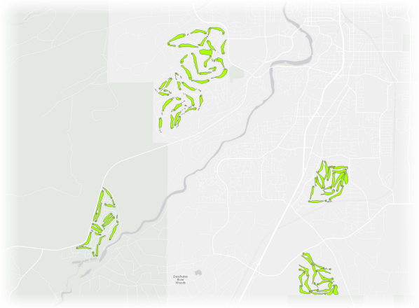
The analysts don't need or want the distance from a river for each fairway or green. So, they decide to create area features encompassing the golf course polygons along with some of the surrounding area. They could just create buffers around the golf course features and dissolve on the name field. One of the analysts recalls, though, that for the Locate Regions tool they can specify a shape for the regions that are created. For example, they can make them more circular or more elliptical. It's possible that golf courses tend to have a particular shape, generally speaking, given their layout. If there turns out to be a predominant shape for the existing courses, they can incorporate that information when they run Locate Regions. Thinking ahead, then, rather than using the Buffer tool they decide to use Directional Distribution, which will create areas that define the shape of each course.
After running the Directional Distribution tool for the golf courses, the analysts can see that while some of the resulting areas are circular, most are in fact elliptical.
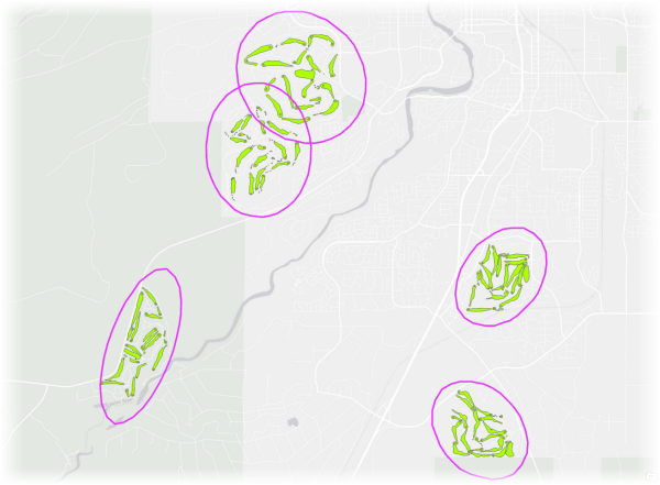
For now what they're interested in is calculating the distance from a river for each of the ellipses representing the golf courses. They see that there are actually two Zonal Statistics tools—one creates an output raster layer representing each of the zones (the ellipses, in this case), while the other creates only a table containing the desired statistics. Since all they really want are the statistics, they choose the latter tool.
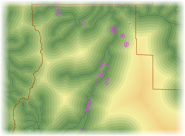

The analysts focus on the minimum distance value in the Zonal Statistics table since that represents the nearest point in the ellipse (representing the golf course environs) to a river. They see that, in fact, 16 of the 22 courses are within a mile of a river. That could be by coincidence rather than design, but the fact remains that the new resort will be competing with these golf courses. And the company's marketing analysts have confirmed through their research that being near a river is a big draw for courses in this relatively arid region. Another three courses are roughly between one and two miles from a river. They decide to stick with their preliminary ranges, assigning values of 5, 3, and 1, from nearest to a river to farthest.
| Miles from river | Suitability value |
|---|---|
0 to 1 | 5 |
1 to 2 | 3 |
>2 | 1 |
Next, they run Zonal Statistics with the distance from airports layer. As with distance from rivers, they decide to focus on the minimum distance value. By this measure, all of the courses are within 20 minutes of an airport, and several are within 5 minutes.

That's helpful—probably an hour from an airport (which was the cutoff they had specified earlier when creating the drive-time areas) is too long, especially since the resort will be competing with the others in the area. They decide on 20 minutes as the maximum suitability—any cells with higher values will be off-limits.
For the rest of the ranges, they'll have to rely on common sense guided by the golf pro's vision for the resort. They know he wants the resort to be somewhat removed from development, so they figure it should be at least a five-minute drive from any airport to make sure the resort is away from noise and traffic. They'll assign cells with a value of 0 to 5 a low suitability value of 1.
They see that 15 of the existing courses (or the greater golf course areas) are within a 15-minute drive of an airport (at their nearest point). To make sure the resort is competitive, they will limit the highest suitability category (a value of 5) to a maximum of 15 minutes. That leaves the 15- to 20-minute range, which gets a mid-suitability rating of 3. They jot down the values just to make sure they've included all the distance values.
| Minutes from airport | Suitability value |
|---|---|
5 to 15 | 5 |
15 to 20 | 3 |
0 to 5 | 1 |
>20 | No Data |
Now all they need to move forward is confirmation from the architect on the slope ranges and suitability values. While they're waiting, the team members do some catch-up on their other projects.
A couple of days later the architect sends back comments (along with an invoice for $1,000). He's created three categories of low slopes. He notes that for typical residential or commercial development, any slopes up to 6 or 7 degrees would be considered very suitable. However, since an important criterion for the golf courses is that they be on flat slopes, he wants to ensure that locations that are essentially flat are scored highest. He assigns very flat slopes (0 to 3 degrees) the highest suitability, somewhat flat slopes (3 to 5 degrees) the next level of suitability, and remaining slopes up to 7 degrees the next level below that. Slopes between 7 to 15 degrees and 15 to 30 degrees comprise the next two categories, while slopes over 30 degrees are deemed not suitable at all.
| Slope in degrees | Suitability value |
|---|---|
0 to 3 | 5 |
3 to 5 | 4 |
5 to 7 | 3 |
7 to 15 | 2 |
15 to 30 | 1 |
>30 | No Data |
With the suitability values for all the layers now set, the analysts reclassify each criteria layer to create a corresponding suitability layer with the new values.
At last they're ready to create the suitability surface by adding the suitability layers together. To do this they'll use the Weighted Sum tool. They could simply add the five layers together, resulting in an output layer with values between 25 and 5. However, Weighted Sum allows them to assign higher weights to layers that are more important.
After a brief discussion the analysts agree that slope is the most important layer—the resort has to be on relatively flat slopes. On the other hand, being near a river and having a view of mountain peaks would be nice, but are not critical. They decide to assign the slope layer a weight of 3 and the other two layers a weight of 1 (that is, no additional importance).
Being near an airport, they decide is fairly important, but not as much as being on flat slopes. They assign this layer a weight of 2. The analysts are split on the last layer—landscape variety. Some feel it's in the same category as views and distance to rivers. Others are adamant that placing the resort among a variety of landscape types is central to the golf pro's vision, and the layer should get a weight equal to distance from airports. In the end the team leader agrees with this argument and decides they will assign the layer a weight of 2.
| Suitability layer | Weight |
|---|---|
Landscape variety | 2 |
Slope | 3 |
Minutes from airport | 2 |
Miles from river | 1 |
View of peaks | 1 |
The team leader specifies the input layers and weights and sets the mask to be the layer of private ownership. The analysts gather around the computer in anticipation while the tool runs. The result looks good.
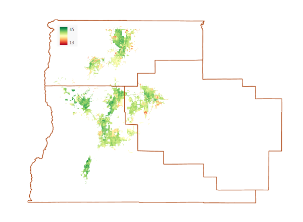
A trial run
While they're reviewing the suitability surface with the input layers, the same analyst who suggested using the existing golf courses to check the proposed suitability criteria suggests that they display the golf course ellipses to see if they correspond to suitable areas.
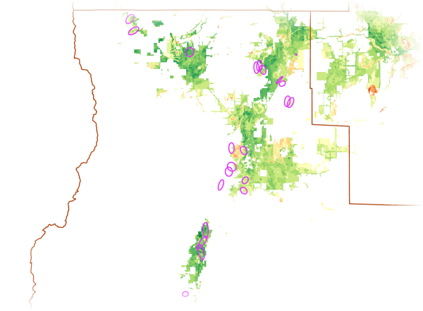
Then she has another thought. What if before running Locate Regions for the two focus counties, they run it for Deschutes County first and see if it chooses the existing golf courses? That would be a good test of how well their analysis is working.
Another team member points out that they used the existing golf courses to help define the criteria for a couple of the layers—distance from rivers and airports—so they'd expect some overlap between the existing courses and the suitable regions identified by the analysis. The team leader concedes the point, but adds that they also used several other criteria in the analysis, and they assigned different weights to the layers. The team members are in general agreement that running this test would be useful.
The team leader assigns the task of running the test to the analyst whose idea it was. The analyst selects Deschutes County and extracts the portion of the suitability surface within it to a new raster. She then opens the Locate Regions tool. There are 22 ellipses, representing the golf courses. She specifies that the tool create 11 regions—that should be enough to see if there is overlap with the courses. She also specifies that the regions be 1,500 acres in size, the size of the future resort.
For this test she's not concerned about the shape of the regions, only whether or not they are coincident with the existing golf courses (represented by the ellipses), so she uses the default shape, which is set to Circle.
When she runs the tool she sees that three regions roughly correspond to existing golf courses—that's pretty good. It means the model is identifying at least some suitable sites. But maybe the analysis can be fine-tuned a bit.
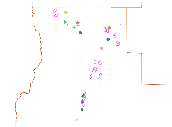
The analyst takes a closer look at the other golf courses to see why those areas weren't selected.
Four of the courses are on public land, so they are located in NoData areas on the suitability surface. Perhaps they are run by a city or by the county, or are run as concessions on publicly owned land. In any case, the development company definitely does not want to get involved in the long-drawn-out process of building on public lands.
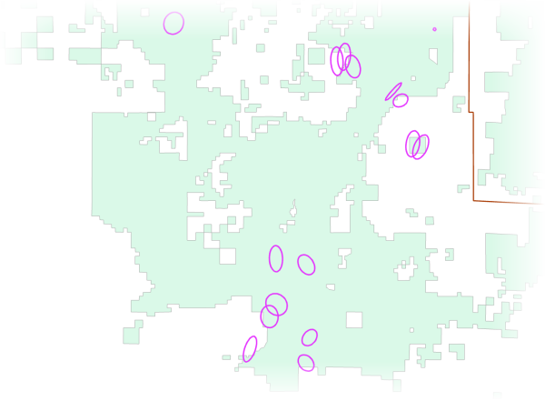
The analyst sees that several other courses, while in otherwise suitable areas, are adjacent to public lands or low-suitability areas, or both, so the Locate Regions tool was likely unable to create regions of the required size in those areas. Fair enough—that's how the analysis is supposed to work. The only way to possibly pick up these areas in the analysis would be to reduce the region size, which they do not want to do.
Of the remaining courses, from the suitability surface the analyst can see that a couple scored in the middle on most of the criteria, so they were likely passed over for higher-scoring regions (clearly, these owners did not do a suitability analysis before building their golf courses).
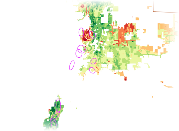
However, a few courses are on areas with low scores on the suitability surface—or even on No Data areas—because they are far from an airport.
The analyst decides to take a closer look at these cases. She sees that several of the courses are more than 20 minutes from an airport—at their farthest point, up to 35 minutes from an airport. Perhaps the original categories—which put the cutoff at 20 minutes—were a bit too conservative. It might be worth revisiting the travel time values to make sure potentially suitable locations are not being eliminated.
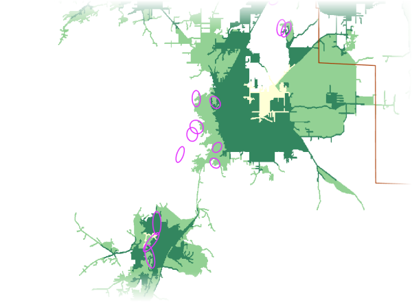
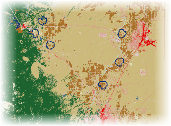
So far she's looked at existing golf courses that did not have corresponding regions created by the analysis. However, there are also several regions that were created where there are no existing courses. She decides to find out what's going on in these areas, as well—some useful information might be revealed.
She finds that in almost all of these cases the regions that were created are located on farmland. This is potentially a problem with the analysis. While in theory farmland might be suitable—it's relatively flat, likely has good soils, and would be easy to clear—the map shows that if the resort were built at one of these locations, it would be surrounded almost exclusively by more farmland, or a mix of farmland and scrub. The analyst is pretty sure that building a resort in the middle of farm fields is not what the golf pro or the developers had in mind.
At this point the team leader decides that there needs to be a meeting to discuss the work so far and what they've learned from the results of the trial run. The analysts meet with development company management as well as the golf pro's people and a representative from the architect's firm.
The development company's management are intrigued by the potential locations that the trial run identified. They'd been leaning toward Deschutes County all along and would be happy to end the analysis right here and look into developing one of these sites. But the golf pro's people are adamant that the project continue and look for suitable sites in the two target counties.
So the discussion turns to the issue of the suitable distance from an airport. Everyone agrees that sites up to 35 minutes from an airport should be considered. The golf pro's team believe that sites within a five-minute drive of an airport should not just be deemed low suitability but should be completely off limits. They cite—yet again—the pro's desire that guests feel that they are away from it all. Ideally, they say, the resort should be a 10- to 20-minute drive from an airport. And sites that are more than 20 minutes away are preferable to ones that are less than 10 minutes.
Moving on, the development team and the pro's people concur that placing the resort in the middle of farmland is not what anybody envisioned. However, they think that completely eliminating these areas might be too drastic a step—there might be some otherwise suitable locations that include a small amount of farmland. So they decide farmland should be kept in the analysis but assigned a low suitability. Since they're on the subject, the architect's representative points out that, in fact, sites that are in or near forest should really be considered the most desirable (even though it might increase construction costs). Having fairways separated by majestic trees will make for a great golf experience. Plus, who doesn't like to go horseback riding in the forest? Everyone agrees.
The analysts realize that in addition to revising the distance from airport suitability values they will need to include an additional suitability layer for land cover. The land-cover layer they are currently including accounts for the variety of land-cover types on and near the potential sites. Now they will also need a layer that indicates how desirable (or suitable) each land-cover type itself is.
After the meeting they set about these tasks. First they update the table showing the drive-time ranges and suitability value for the distance from airports layer, and create the revised suitability layer.
| Minutes from airport | Suitability value |
|---|---|
10 to 20 | 5 |
20 to 35 | 3 |
5 to 10 | 1 |
0 to 5 | NoData |
>35 | NoData |
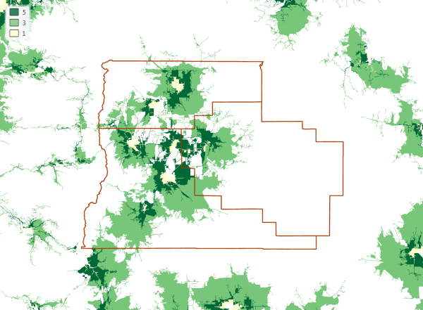
They then list the land-cover categories and corresponding suitability values. This will be based on a somewhat subjective interpretation of how desirable the land-cover type is as a location for the resort. Any land-cover type that is not suitable for a new development will be off limits and assigned NoData. They quickly put the lands with existing development in this category, along with perennial snow and ice and barren lands.
While it might be nice to have lakes or ponds at or near the resort, they can't actually build on these. In any case, the architect will design water hazards for the courses and other water features for the resort. So open water also gets a value of NoData.
Now they consider the other land-cover types. It's already been agreed that the three forest types will be assigned a value of 5 and cultivated crops a value of 1. They also assign the two wetland types a value of 1—while they might be interesting to look at, trying to build, or even get permission to build, on or near wetlands will be next to impossible.
The other categories—shrub and scrub, herbaceous (grassland), and pasture—while not the most desirable, would be acceptable, especially if they are mixed in with forest. And, they would require little clearing for construction. The analysts assign these types a value of 3.
| Land-cover type | Suitability value |
|---|---|
Deciduous Forest | 5 |
Evergreen Forest | 5 |
Mixed Forest | 5 |
Shrub/Scrub | 3 |
Herbaceous | 3 |
Hay/Pasture | 3 |
Cultivated Crops | 1 |
Woody Wetlands | 1 |
Emergent Herbaceous Wetlands | 1 |
All Other Categories | NoData |
They then create the land-cover suitability layer.
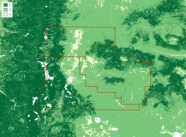
With the final suitability layers ready to go, they can run the analysis to find suitable sites in the two target counties.
The final analysis
The analysts now have an additional layer—land-cover suitability—to assign a weight to. After reviewing the weights they used last time, the team leader, in a reversal, decides that in light of the relative importance of the new land-cover suitability layer, they should assign the landscape variety layer a weight of 1 (instead of 2). This layer now seems to be comparable in importance to views and distance from rivers—a nice amenity but not a deal breaker. They will assign the land-cover suitability layer a weight of 2, comparable to distance from airports.
| Suitability layer | Weight |
|---|---|
Landscape variety | 1 |
Slope | 3 |
Minutes from airport | 2 |
Miles from river | 1 |
View from peaks | 1 |
Land cover | 2 |
The team leader uses the Weighted Sum tool to create the new suitability layer and extracts the portion of the layer that falls within the two preferred counties.
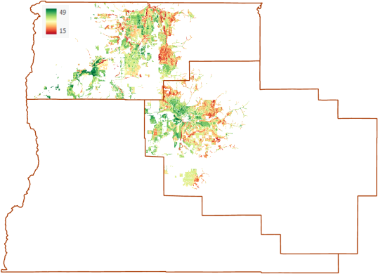
Now she can run Locate Regions to identify suitable sites. The original goal was to identify at least five suitable sites. She specifies seven, just to provide a few more options. She also specifies the shape for the regions to be elliptical, based on what the analysts found when they created the areas around existing golf courses. But, since the shape is less important than finding the most suitable sites, she gives preference to suitability over shape (that is, it's more important that the regions have a high suitability score than that they are elliptical). Also, since the developers are looking to choose a single site, she specifies a selection method of Sequential so that the regions are ranked by overall suitability. (The other option—Combinatorial—will select the best combination of seven sites, not what the developers are looking for in this case.)
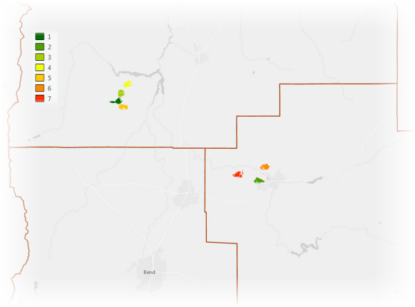
The results are interesting. Rather than creating seven widely dispersed regions, Locate Regions identifies two areas where the regions cluster—one in Jefferson County and one in Crook County. The analysts now know that there are at least several 1,500-acre contiguous blocks of land in each of these areas that are very suitable for the resort.
In addition, Locate Regions assigns a score to each region—the region with the highest overall suitability is assigned a score of 1; the one with the second highest overall suitability, 2; and so on. The analysts see that the higher-scoring regions are mainly located in Jefferson County.
The analysts put together a story map showing the results, along with an explanation of the criteria that went into the analysis. They include a couple of 3D scenes of the regions and surrounding landscape so the golf pro can see which sites best match his original vision.
The best-laid plans
After reviewing the results, the development company managers begin negotiating the path forward with the golf pro and his people, including the golf course architect.
The pro wants to build in western Jefferson County—this area has a much more dramatic landscape and is more off the beaten path. It's exactly the type of location he had envisioned. Plus, he points out, the sites in this area scored higher in the analysis. The development company prefers the sites in Crook County, which are closer to highways, towns, and the main city in the area, which offers additional amenities. They figure word of mouth will spread much faster if their resort isn't out in the middle of nowhere.
While the negotiations are ensuing, the development company starts checking into property acquisition in the two potential areas. They quickly discover that word has already leaked about the new resort. Not only that, but apparently a New York-based real estate developer that has developed high-end golf courses throughout the world has also been making inquiries about property in Jefferson County. So, not surprisingly, land prices have suddenly seen a dramatic increase.
At this point, the golf pro starts having second thoughts. The project requires three times as much land as he first thought, and now land prices are going up. Unbeknownst to his business partners at the development company, the owners of one of the existing resorts in the area have approached the pro about a licensing deal. All he'd have to do is agree to have his name attached to their resort, and show up for a tournament once a year. He decides to pull out of the development project and take the deal. When informed of this outcome by the pro's legal team, the development company sues the pro for breach of contract. The pro files a countersuit for theft of intellectual property (his argument is that the site selection process was based mainly on his knowledge of golf course design and the industry in general).
The other investors see that their worst fears have come true, and they also pull out of the project. While the lawsuits move forward, the development company decides to go ahead with a scaled-down project—a single golf course with a clubhouse and upscale restaurant. They will take a closer look at the sites in Crook County, as well as the sites identified by the trial run in Deschutes County (which was, in fact, their initial preference).