Mit der Geostatistical Analyst-Lizenz verfügbar.
Before you produce the final surface, you should have some idea of how well the model predicts the values at unknown locations. Cross-validation and validation help you make an informed decision as to which model provides the best predictions. The calculated statistics serve as diagnostics that indicate whether the model and/or its associated parameter values are reasonable.
Cross-validation and validation use the following idea—remove one or more data locations and predict their associated data using the data at the rest of the locations. In this way, you can compare the predicted value to the observed value and obtain useful information about the quality of your kriging model (for example, the semivariogram parameters and the searching neighborhood).
Cross-validation
Cross-validation uses all the data to estimate the trend and autocorrelation models. It removes each data location one at a time and predicts the associated data value. For example, the diagram below shows 10 data points. Cross-validation omits a point (red point) and calculates the value at this location using the remaining 9 points (blue points). The predicted and actual values at the location of the omitted point are compared. This procedure is repeated for a second point, and so on. For all points, cross-validation compares the measured and predicted values. In a sense, cross-validation "cheats" a little by using all the data to estimate the trend and autocorrelation models. After completing cross-validation, some data locations may be set aside as unusual if they contain large errors, requiring the trend and autocorrelation models to be refit.

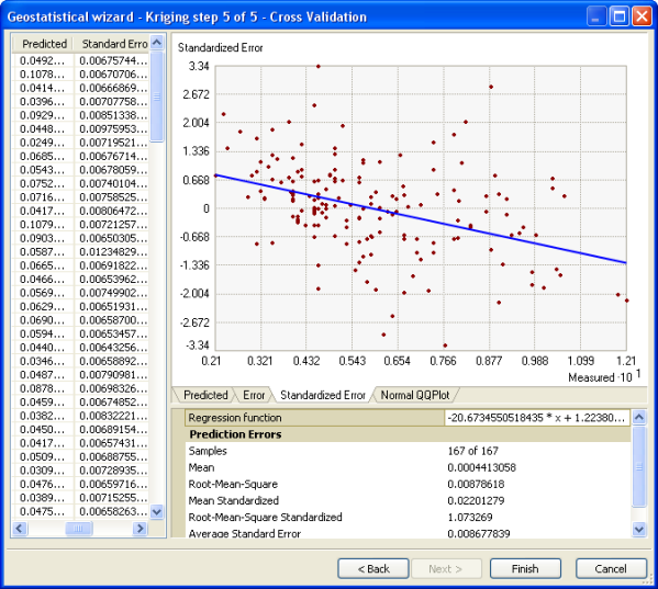
Cross-validation is performed automatically, and results are shown in the last step of the Geostatistical Wizard. Cross-validation can also be performed manually using the Cross Validation geoprocessing tool.
Validation
Validation first removes part of the data (call it the test dataset) then uses the rest of the data (call it the training dataset) to develop the trend and autocorrelation models to be used for prediction. In Geostatistical Analyst, you create the test and training datasets using the Subset Features tool. Other than that, the types of graphs and summary statistics used to compare predictions to true values are similar for both validation and cross-validation. Validation creates a model for only a subset of the data, so it does not directly check your final model, which should include all available data. Rather, validation checks whether a protocol of decisions is valid, for example, choice of semivariogram model, lag size, and search neighborhood. If the decision protocol works for validation, you can feel comfortable that it also works for the entire dataset.
Model validation can be performed using the GA Layer to Points geoprocessing tool. For more information on how to validate a model, see Using validation to assess models.
Plots
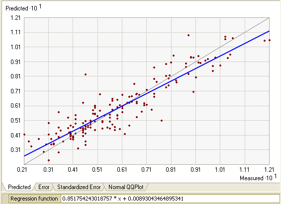
Geostatistical Analyst gives several graphs and summaries of the measured values versus the predicted values. A scatterplot of predicted values versus true values is given. You might expect that these should scatter around the 1:1 line (the black dashed line in the plot given below). However, the slope is usually less than 1. It is a property of kriging that tends to underpredict large values and overpredict small values, as shown in the following figure:

The fitted line through the scatter of points is given in blue with the equation given just below the plot. The error plot is the same as the prediction plot, except the measured values are subtracted from the predicted values. For the standardized error plot, the measured values are subtracted from the predicted values and divided by the estimated kriging standard errors. All three of these plots show how well kriging is predicting. If all the data was independent (no autocorrelation), all predictions would be the same (every prediction would be the mean of the measured data), so the blue line would be horizontal. With autocorrelation and a good kriging model, the blue line should be closer to the 1:1 (black dashed) line. The regression equation below each of these three plots is calculated using a robust regression equation. This procedure first fits a standard linear regression line to the scatterplot. Next, any points that are more than two standard deviations above or below the regression line are removed, and then a new regression equation is calculated. This procedure ensures that a few outliers will not corrupt the entire regression equation.
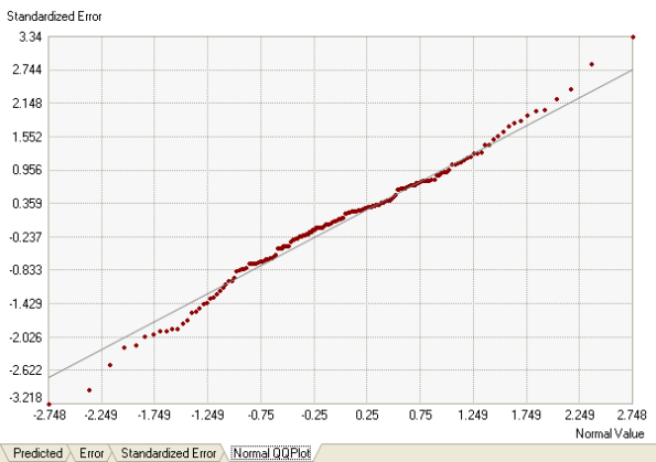
The final plot is a QQ plot. This shows the quantiles of the difference between the predicted and measured values and the corresponding quantiles from a standard normal distribution. If the errors of the predictions from their true values are normally distributed, the points should lie roughly along the gray line. If the errors are normally distributed, you can be confident in using methods that rely on normality (for example, quantile maps in simple kriging).

Prediction error statistics
Finally, some summary statistics on the kriging prediction errors are given below. Use these as diagnostics. These diagnostics can be calculated with the Cross Validation tool or the Geostatistical Wizard.
- You would like your predictions to be unbiased (centered on the true values). If the prediction errors are unbiased, the mean prediction error should be near zero. However, this value depends on the scale of the data; to standardize these, the standardized prediction errors give the prediction errors divided by their prediction standard errors. The mean of these should also be near zero.
- You would like your assessment of uncertainty, the prediction standard errors, to be valid. Each of the kriging methods gives the estimated prediction kriging standard errors. In addition to making predictions, you estimate the variability of the predictions from the true values. It is important to get the correct variability. For example, in ordinary, simple, universal, and empirical Bayesian kriging (assuming the data is normally distributed), the quantile and probability maps depend on the kriging standard errors as much as the predictions themselves. If the average standard errors are close to the root mean squared prediction errors, you are correctly assessing the variability in prediction. If the average standard errors are greater than the root mean squared prediction errors, you are overestimating the variability of your predictions. If the average standard errors are less than the root mean squared prediction errors, you are underestimating the variability in your predictions. Another way to look at this is to divide each prediction error by its estimated prediction standard error. They should be similar, on average, so the root mean squared standardized errors should be close to 1 if the prediction standard errors are valid. If the root mean squared standardized errors are greater than 1, you are underestimating the variability in your predictions; if the root mean squared standardized errors are less than 1, you are overestimating the variability in your predictions.
