Mit der Geostatistical Analyst-Lizenz verfügbar.
You can assume that as locations get farther from the prediction location, the measured values have less spatial autocorrelation with the prediction location. As these points have little or no effect on the predicted value, they can be eliminated from the calculation of that particular prediction point by defining a search neighborhood. It is also possible that distant locations may have a detrimental influence on the predicted value if they are located in an area that has different characteristics than those of the prediction location. A third reason to use search neighborhoods is for computational speed. If you have 2,000 data locations, the matrix would be too large to invert, and it would not be possible to generate a predicted value. The smaller the search neighborhood, the faster the predicted values can be generated. As a result, it is common practice to limit the number of points used in a prediction by specifying a search neighborhood.
The specified shape of the neighborhood restricts how far and where to look for the measured values to be used in the prediction. Additional parameters restrict the locations that are used within the search neighborhood. The search neighborhood can be altered by changing its size and shape or by changing the number of neighbors it includes.
The shape of the neighborhood is influenced by the input data and the surface that you are trying to create. If there are no directional influences in the spatial autocorrelation of your data (see Accounting for directional influences for more information), you will want to use points equally in all directions, and the shape of the search neighborhood is a circle. However, if there is directional autocorrelation or a trend in the data, you may want the shape of your neighborhood to be an ellipse oriented with the major axis parallel to the direction of long-range autocorrelation (the direction in which the data values are most similar).
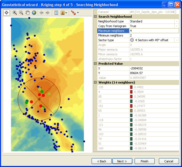
The search neighborhood can be specified in the Geostatistical Wizard., as shown in the following example:
- Neighborhood type: Standard
- Maximum neighbors = 4
- Minimum neighbors = 2
- Sector type (search strategy): Four Sectors with 45° offset; radius = 182955.6
- Coordinates of test point (x = -2084032, y = 89604.57)
- Predicted value = 0.08593987

The Weights section lists the weights that are used to estimate the value at the location marked by the crosshair on the preview surface. The data points with the largest weights are highlighted in red.
Once a neighborhood shape is specified, you can restrict which locations within the shape should be used. You can define the maximum and minimum number of neighbors to include and divide the neighborhood into sectors to ensure that you include values from all directions. If you divide the neighborhood into sectors, the specified maximum and minimum number of neighbors is applied to each sector.
There are several different sector types that can be used:

- One sector
- Ellipse with four sectors
- Ellipse with four sectors and a 45-degree offset
- Eight sectors
Kriging uses the data configuration specified by the search neighborhood in conjunction with the fitted semivariogram model; weights for the measured locations can be determined. Using the weights and the measured values, a prediction can be made for the prediction location. This process is performed for each location within the study area to create a continuous surface. Other interpolation methods follow the same process, but the weights are determined using techniques that do not involve a semivariogram model.
The maximum number of neighbors that can be used depends on the interpolation method. For a single sector, the maximum number of neighbors for each method is as follows:
- Areal Interpolation—200 neighbors
- Diffusion Interpolation with Barriers—No limit on number of neighbors
- Empirical Bayesian Kriging—64 neighbors
- Global Polynomial Interpolation—Does not use a searching neighborhood
- Inverse Distance Weighted—1,000 neighbors
- Kernel Interpolation with Barriers—No limit on number of neighbors
- Kriging (other than Empirical Bayesian Kriging)—200 neighbors
- Local Polynomial Interpolation—1,000 neighbors
- Radial Basis Functions—64 neighbors
The maximum number of neighbors is affected when different numbers of sectors are used; for example, when four sectors are used, divide the number of neighbors by four, and for eight sectors, divide the number by eight.
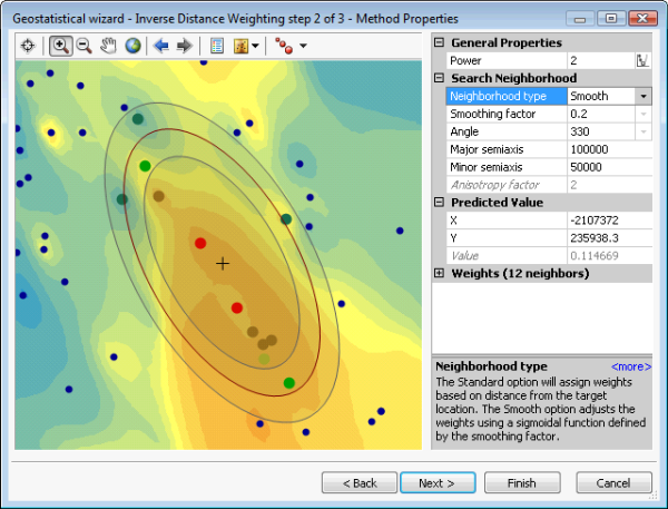
The Smooth Interpolation option creates three ellipses. The central ellipse uses the Major semiaxis and Minor semiaxis values. The inner ellipse uses these semiaxis values multiplied by 1 minus the value for Smoothing factor, whereas the outer ellipse uses the semiaxis values multiplied by 1 plus the smoothing factor. All the points within these three ellipses are used in the interpolation. Points inside the smallest ellipse have weights assigned to them in the same ways as for standard interpolation (for example, if the method being used is inverse distance weighted interpolation, the points within the inner ellipse are weighted based on their distance from the prediction location). The points that fall between the inner ellipse and the outer ellipse get weights as described for the points falling inside the inner ellipse, but then the weights are multiplied by a sigmoidal value that decreases from 1 (for points located just outside the inner ellipse) to 0 (for points located just outside the outer ellipse). Data points outside the outer ellipse have zero weight in the interpolation. An example of this is shown below:

The exceptions to the above descriptions are as follows:
- Areal interpolation, which only supports one sector.
- Empirical Bayesian kriging, which requires a circular search neighborhood; therefore, Major semiaxis and Minor semiaxis have been replaced with Radius. The value of the radius represents the length of the radius of the searching circle.
In Geostatistical Analyst, the weights for all nonkriging models are defined by a priori analytic functions based on the distance from the prediction location. Most kriging models predict a value using the weighted sum of the values of the nearby locations. Kriging uses the semivariogram to define the weights that determine the contribution of each data point to the prediction of new values at unsampled locations. Because of this, the default search neighborhood used in kriging is constructed using the major and minor ranges of the semivariogram model.
It is expected that a continuous surface is made from continuous data, such as temperature observations. However, all interpolators with a local searching neighborhood generate predictions (and prediction standard errors) that can be substantially different for nearby locations if the local neighborhoods are different. To see a graphical representation of why this occurs, see Smooth interpolation.