Mit der Geostatistical Analyst-Lizenz verfügbar.
Geostatistical layers can be converted into raster format using the GA Layer to Grid geoprocessing tool in the Geostatistical Analyst toolbox (see An overview of the Working with Geostatistical Layers toolset). You can also open this tool by right-clicking the layer in the ArcMap table of contents and using the Data > Export to Raster option.
Block interpolation is used when creating a raster from a geostatistical layer. Block interpolation is an interpolation method that predicts the average value of a phenomenon within a specified area. For empirical Bayesian kriging and all other non-kriging methods, block interpolation works by calculating predictions for a number of specified locations within an area; the values are averaged, and the average is assigned as the prediction for the entire area. For example, if you specify 10 locations to be predicted within an area, predictions will be made for each of the 10 locations using an identified interpolation model and the original sample points collected for the phenomenon.
For kriging methods (other than empirical Bayesian kriging) the value of the raster cell is calculated according to the standard block kriging equations (see the reference at the end of this topic). If a transformation is used, the standard block kriging equations are applied to the transformed data, and a correction is applied during back transformation. However, after back transformation, these block predictions may be biased, and the recommended methodology in this case is to use simulations with the Gaussian Geostatistical Simulations geoprocessing tool.
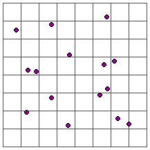
When converting a geostatistical layer to a raster, the shapes of the blocks performing the averaging are within individual raster cells. The following diagram shows sample points with the block configuration (the raster) that will be used in the block interpolation:

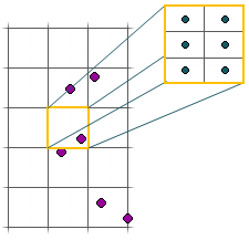
In the conversion, you specify how many point prediction locations within each cell to use in the averaging. For example, you can specify predictions for two points in the x direction and three points in the y direction for each cell. The prediction points will be distributed within each cell so that they represent (or influence) the same amount of area. Thus, no weighting will occur for any of the prediction points. The prediction points are located in the center of each subunit—in this case, in the center of each of the six blocks.
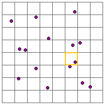
In the following diagram, the highlighted cell will be used to demonstrate block interpolation for a single cell (or block) in the raster. This procedure is applied to each cell in the output raster.

The following diagram is a close-up of the highlighted block in the previous diagram. A prediction will be made for each of the six points in the cell using the interpolation model identified in the geostatistical layer and the original sample points. The six predictions will be averaged and assigned to that cell.

If you only specify one point in the x direction and one in the y direction, you'll make the prediction for the center of each output cell. Processing times will increase as the number of prediction points increases.
The reason you may have more prediction points in either the x or y direction is to account for directional trends. In the 2-by-3 example above, the spacing of the prediction points in the north–south direction is closer than in the east–west direction. Having more prediction points in the north–south direction increases the sampling in that direction to capture the higher variability. That is, the values of the phenomenon change quicker in the north–south direction than in the east–west direction. To capture this, you'll need more sample points in that direction.
References
- Chiles, J.P. and Delfiner, P., Geostatistics: Modeling Spatial Uncertainty, John Wiley & Sons, New York (1999), Section 3.5 (pp. 203-211)