Exercise 4: Finding an alternate access route

Available with Spatial Analyst license.

Complexity:

Beginner

Data Requirement:

ArcGIS Tutorial Data for Desktop

In this exercise, you'll find the best route for a new access road from the optimal school location site to a nearby road intersection. The steps you might follow to produce such a path are outlined below.

• Create the source dataset if necessary. The source is the school site (the final_site feature class) you created in exercise 3.
• Create the cost dataset by deciding which datasets are required, reclassifying them to a common measurement scale, weighting them, then combining them.
• Perform cost distance analysis using the source and cost datasets as inputs. The distance dataset created from this tool is a raster in which the value of each cell is the accumulated cost of traveling from each cell back to the source.

  To find the least costly path, you need a direction dataset, which can be created as an additional dataset using the Cost Distance tool. This gives you a raster of the direction of the least costly path from each cell back to the source (in this exercise, the school site).

• Create the destination dataset if necessary. In this exercise, the destination dataset is a point at a road junction.
• Perform cost path analysis using the distance and direction datasets created with the Cost Distance tool.

This exercise will take approximately 30 minutes to complete. Start this exercise with your Site Analysis map document created in the previous exercise open.

Creating a new model

You'll create a new model, Find Best Route, inside your Site Analysis Tools toolbox. This model will calculate the best path through the landscape from the source (the school site) to the destination point, taking into consideration the slope of the land and the type of land use the path will cross.

Setting up the model

1. Right-click the Site Analysis Tools toolbox and click New > Model.

Renaming the model

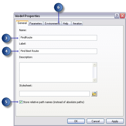
1. On the main menu, click Model > Model Properties.

   Note:

   The model properties and environments will be set as they were in the previous exercise.

2. Click the General tab and type FindRoute in the Name text box.
3. Type Find Best Route in the Label text box.
4. Check Store relative path names (instead of absolute paths).

   

Specifying environment settings

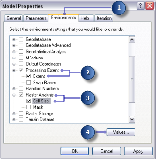
1. Click the Environments tab.
2. Expand Processing Extent and check Extent.
3. Expand Raster Analysis and check Cell Size.
4. Click Values.

   

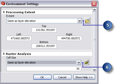
5. Expand Processing Extent. Set the Extent by clicking the drop-down arrow and selecting Same as Layer elevation.
6. Expand Raster Analysis. Set the Cell Size by clicking the drop-down arrow and selecting Same as Layer elevation.
7. Click OK on the Environment Settings window.

   

8. Click OK on the Model Properties window.
9. On the toolbar, click the Save button .

Creating the cost dataset

You created the source dataset, final_site, and a slope dataset, Slope Output, in the previous exercise. You'll create the cost dataset that will identify the cost of traveling over the landscape from any location back to the proposed new school site, based on the fact that it is costlier to traverse steep slopes and construct a road on certain land-use types.

This section of your model will look like the following:

Setting up the model

1. Add Slope Output to your model.
2. Locate the Reclassify tool and add it to ModelBuilder in line with Slope Output.
3. Click the Add Connection tool . Use the connect tool to connect Slope Output to the Reclassify tool.
4. Click the Select tool on the model toolbar.

Reclassifying slope

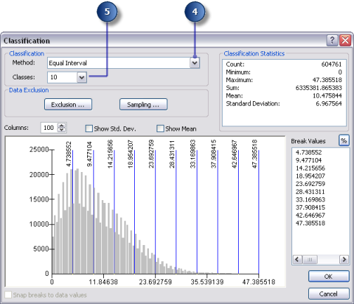
It is preferable that the new road traverses less steep slopes. You will reclassify the Slope Output layer, slicing the values into equal intervals. You'll assign a value of 10 to the most costly slopes (those with the steepest angle of slope) and 1 to the least costly slopes (those with the least angle of slope) and rank the values in between linearly.

1. Open the Reclassify tool.
2. Accept the default for the Reclass field parameter so the Value field will be used.
3. Click Classify.

   

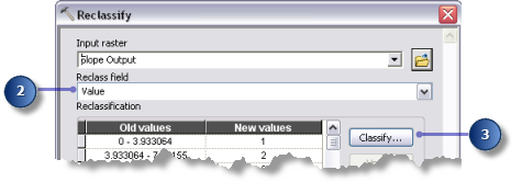
4. Click the Method drop-down arrow and click Equal Interval.
5. Click the Classes drop-down arrow and click 10.

   You want to avoid steep slopes when constructing the road, so steep slopes should be assigned higher values in the cost dataset. Because the default assigns higher values to steeper slopes, you do not need to change the default New values.

6. Click OK.

   

7. Accept the default for the Output raster parameter.
8. Click OK.
9. Rename the output variable from the Reclassify tool to Reclassed slope.
10. Right-click the Reclassify tool and click Run.

Weighting and combining datasets

You will now combine the Reclassed slope and landuse datasets to produce a dataset of the cost of building a road through each location in the landscape, in terms of steepness of slope and land-use type. In this model, each dataset has equal weight.

1. Locate the Weighted Overlay tool and add it to ModelBuilder in line with Reclassed slope.
2. Open the Weighted Overlay tool.

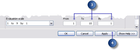
   The default evaluation scale is from 1 to 9 by 1. As in exercise 3, a scale of 1 to 10 was used when reclassifying the slope dataset, so before adding input rasters to the tool, you'll set the evaluation scale from 1 to 10 by 1. This means you will avoid having to update the scale values after adding your input slope dataset.

3. Type 1, 10, and 1 in the From, To, and By text boxes.
4. Click Apply.

   

5. Click the Add raster row button . For the Input raster, select Reclassed slope variable from the drop-down list and leave the Input field as Value. Click OK.
6. Click the Add raster row button . This time, add the landuse layer. Set the Input field to Landuse and click OK.

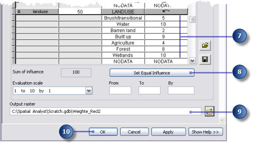
   You'll weight the scale values of the landuse layer so they are comparable with your Reclassed slope dataset. A higher value indicates that it is costlier to build a road through a particular land-use type.

7. Type the following Scale Values:
   • Brush/transitional—5
   • Water—10
   • Barren land—2
   • Built up—9
   • Agriculture—4
   • Forest—8
   • Wetlands—10

   Caution:

   Be cautious when using Restricted for the scale value when creating a cost surface. Using Restricted assigns a value to the cell that is the minimum value of the evaluation scale minus 1 (zero in this exercise), so your restricted areas will appear to be assigned the lowest cost when they are actually excluded from the analysis. Cells with this value should be rendered appropriately to avoid confusion. You could, instead, assign a high cost or set the scale value to NoData for areas you want to exclude from the analysis. If NoData is used, check first that there are no areas of NoData in your input rasters. If there are, it will be difficult to tell whether an area of NoData is there because it was excluded or there was no original information at that location for one of your inputs.

8. You will now assign an equal percentage of influence to each raster, since they are both equally important in this analysis. Click Set Equal Influence to assign an equal percentage of influence (50 percent each) to each input raster.
9. Accept the default for the Output Raster.
10. Click OK.

    

Executing Weighted Overlay

1. Click the Auto Layout button , then click the Full View button .
2. Rename the output variable from the Weighted Overlay tool to Cost surface and click OK.
3. Right-click the Cost surface variable and click Add To Display.
4. Run the Weighted Overlay tool.
5. On the toolbar, click the Save button .

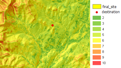
Examine the layer added to your ArcMap display. Locations with low values indicate areas that will be the least costly to build a road through.

Cost-surface map

Finding the least costly path

To find the least costly path between the site for the new school, identified in exercise 3, and the destination site, the Cost Distance tool and the Cost Path tool will be used. There are two outputs from the Cost Distance tool. The Output distance raster shows the accumulated cost of traveling from any location (or cell) to the source (the school site). It does not contain information on which way to travel from a particular cell to the source, just how much it will cost to get there following the least costly path. The Output backlink raster shows which way to travel from any cell, following the least costly path back to the source. Using these outputs as inputs to the Cost Path tool, along with input destination data, you will calculate the least cost path between the site for a new school and the destination site.

Setting up the model

1. Add the final_site and the destination layers to ModelBuilder.
2. Add the Cost Distance and the Cost Path tools to ModelBuilder.

   Both the Cost Distance and the Cost Path tools are located in the Spatial Analyst Tools toolbox in the Distance toolset.

   

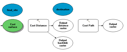
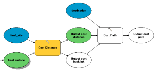
3. Use the Add Connection tool to connect final_site and Cost surface to the Cost Distance tool.
4. Rename the Output distance raster variable to Output cost distance and rename the Output backlink raster variable to Output cost backlink.
5. Use the Add Connection tool to connect destination, Output cost distance, and Output cost backlink to the Cost Path tool.
6. Rename Output raster to Output cost path.
7. On the model toolbar, click the Select tool , the Auto Layout button , and the Full View button .

   

Setting Cost Distance parameters

You will now run the Cost Distance tool using the cost dataset you just created (which identifies the cost of traveling through each cell) and the final_site layer (the source) you created in exercise 3. The outputs from this tool are a distance dataset in which each cell contains a value representing the accumulated least cost of traveling from that cell to the source and a backlink dataset that gives the direction of the least costly path from each cell back to the source.

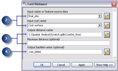
1. Open the Cost Distance tool.
2. Confirm that the Input raster or feature source data is the final_site layer and that the Input cost raster is Cost surface variable.
3. Accept the defaults for the Output distance raster and the Maximum distance.
4. Type cost_bklink for the name of the Output backlink raster.

   By default, the path to the scratch workspace (C:\Spatial Analyst\Scratch.gdb) will automatically be appended in front of the dataset name you just entered for the Output backlink raster.

5. Click OK.

   

Setting Cost Path parameters

The Cost Distance tool outputs a distance raster and a backlink raster, each of which are used in the Cost Path tool. The destination layer was provided, and the layer is the starting point for the new road to the school site.

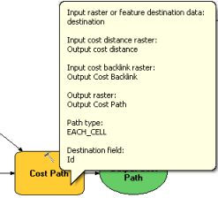
1. Hover over the Cost Path tool to verify that the parameters have the correct input datasets.
   • Input raster or feature destination data is set to the destination layer.
   • Input cost distance raster is set to the Output cost distance variable.
   • Input cost backlink raster is set to the Output cost backlink variable.

2. Accept the default for the Output raster, the Path type, and the Destination field parameters.

   When the input feature destination data is processed, it will be converted temporarily to a raster as part of the processing. There will only be one cell in this raster, because there is only one destination point. The value for the Path type parameter can be left as EACH_CELL. Only one path will be created, since there is only one cell.

   

Running the cost distance analysis

1. Right-click the Output cost distance, Output cost backlink, and Output cost path variables and click Add To Display.
2. Run the Find Best Route model.

Examine the layers added to your ArcMap display. The Output cost path layer represents the least costly path from the school site to the destination point. It avoids steep slopes and certain land-use types that are considered costlier for constructing the road.

Raster to Polyline

Set parameters for Raster to Polyline

As a last step in your model, you'll convert the raster path to a polyline for display.

1. Remove the created layers Slope output, Reclassed slope, Cost surface, Output cost distance, and Output cost backlink so you can see the path displayed over the landuse and hillshd layers.
2. Add the Raster To Polyline tool to ModelBuilder.

   The Raster To Polyline tool is in the Conversion Tools toolbox in the From Raster toolset.

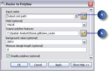
3. Open the Raster To Polyline tool.
4. Click the Input raster drop-down arrow and select the Output cost path variable.
5. Leave the Field parameter as VALUE.
6. Click the Browse button next to the Output polyline features parameter and navigate to your Stowe file geodatabase C:\Spatial Analyst\Stowe.gdb.
7. Type new_route for the Name of the feature class and click Save.
8. Accept the defaults for all other parameters and click OK.

   

Run Raster to Polyline

1. Click the Auto Layout button , then click the Full View button .
2. Rename the new_route output variable to Output route.
3. Right-click the Output route variable and click Add To Display.
4. Run the Raster To Polyline tool.

Examine the new_route layer that is added to your ArcMap display. The raster path has been converted to a polyline.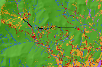

Map with the polyline representing the new route

You can easily change parameter values to experiment with different outcomes and rerun the model. Only the processes in the model that are dependent on the output of the altered process will need to be rerun. For example, lowering the weight applied to cell values where the landuse is Built up from 9 to 1 will alter the potential path for the new road considerably—it will tend to follow existing roads where it can, which may be a less costly option to consider.

Saving the map document

You have set relative paths for both models created in this tutorial, so if the toolbox containing the models and the data is moved (keeping the same structure between them) to a new location on disk, the paths to the data sources will be set relative to the position of the toolbox. By default, your map document is set to store relative path names to data sources.

1. On the toolbar, click the Save button .
2. Click File > Exit.

Summary

This brings you to the end of this tutorial. You have been introduced to some of the tools available with ArcGIS Spatial Analyst extension, both through the Spatial Analyst toolbar and the Spatial Analyst Tools toolbox. You've learned how to build models that are reusable and can be shared with others. In particular, you've learned how to create a suitability map, and you've learned how to calculate the least costly path across a landscape. The sequences of steps involved can be applied to many different applications.

Feedback on this topic?