Available with Spatial Analyst license.
Solute transport in a porous medium involves two principal mechanisms: advection and hydrodynamic dispersion. Advection describes the passive transport of a solute with the transporting fluid. Dispersion is the mixing of the solute with the fluid by differential movement of the fluids through pore spaces. Porous Puff assumes the aquifer is vertically mixed—that is, the concentration is the same throughout a vertical section. This allows the application of a mathematical model in two dimensions, as required by the raster data model.
Two-dimensional dispersion
Two-dimensional dispersion in a porous medium is governed by the advection–dispersion equation (Bear, 1979; Freeze and Cherry, 1979; and Marsily, 1986), written in terms of longitudinal (in the direction of flow) and transverse (perpendicular to the direction of flow) directions XL and XT, respectively, as:

- where:
C : The concentration of the solute as a function of two spatial dimensions and time t.
∂C/∂t : Represents the time derivative.
D'L : The effective (retarded) dispersion coefficients in the longitudinal direction.
D'T : The effective (retarded) dispersion coefficients in the transverse direction.
λ : The decay coefficient, assumed to be a constant for first-order exponential decay.
Dispersion coefficients
The dispersion coefficient is a measure of the extent to which the solute spreads in the specified direction:
D'i = Di/R
- where:
R : The retardation factor.
i : The direction (longitudinal or transverse).
The dispersion coefficient is related to the behavior of the solute in a particular medium.
Relationship between dispersivity and dispersion coefficient
The dispersivities αL (longitudinal dispersivity) and αT (derived from the dispersivity ratio) are related to the dispersion coefficients by:
D'L = αL V' and
D'T = αT V'
where:
V' : The average retarded velocity of the puff.
XL : The displacement in the longitudinal direction, parallel to the direction of flow at the centroid of mass.
XT : The displacement in the transverse direction, perpendicular to the direction of flow at the centroid of mass.
V'L : The retarded solute velocity in the longitudinal direction.
In groundwater flow:
V = q / n
- where:
q : The Darcy flux (discharge per cross-sectional area).
n : The effective porosity of the geologic formation.
V' = V / R
Refer to the documentation for Darcy Velocity for a more detailed discussion of transport velocities.
Gaussian dispersion
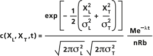
The approximate solution to this equation used in Porous Puff is based on the assumption of Gaussian dispersion of an instantaneous point source in a two-dimensional domain with an initial concentration of zero (for example, a clean, vertically mixed aquifer), and is calculated by the following equation:

- where:
M : The mass of solute released instantaneously at the source, in units of mass.
n : The aquifer porosity.
R : The retardation factor.
b : The aquifer thickness in units of length.
 : the variance of the Gaussian distribution in the longitudinal and transverse directions, determined as a function of the longitudinal dispersivity and dispersivity ratio you provide and the length of the travel path of the center of mass of the solute obtained from the track file.
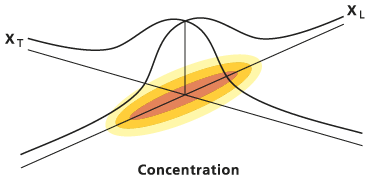
The general elliptical shape of this bivariate Gaussian distribution function is illustrated below:

There are several notable limitations to and assumptions implied in the Porous Puff solution. The dispersion ellipse is centered in the mass of the solute, which is assumed to have moved along the flow track described in the input file. The orientation of the ellipse is fixed to the flow track as well, with the principal axis tangent to the track at the centroid. The porosity and thickness, which also contribute to the distribution, are interpolated from their respective rasters at the centroid, incorporating no information from the surrounding cells. Retardation, time, decay coefficient, longitudinal dispersivity, and dispersivity ratio are supplied as constants by you.
Dispersivity
The dispersivity is a parameter governing the dispersion of a solute through a porous medium and is specified in units of length. In the Porous Puff model, the dispersivity is used to calculate the variance  of the Gaussian dispersion equation above, according to:
 and
and 
The nature of dispersivity and methods for its determination are topics of intense interest and controversy in the groundwater modeling community, and there is no universally accepted way to estimate its values. A discussion of dispersivities in various geologic formations can be found in Gelhar et al. (1992).
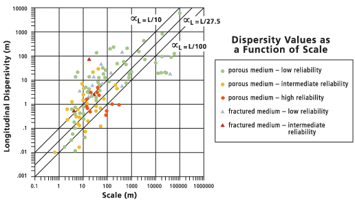
The following graph summarizes a variety of data from the published literature and relates longitudinal dispersivity to the scale of the problem of interest, meaning the distance from the source location to the point of observation.

The solid line (the center line) in the graph represents the default value for longitudinal dispersivity calculated by the Porous Puff tool.
The line is created from a linear regression fit of
 to L resulting in
  or
or  , in which the length of the travel path L is the observation scale.
The statistics of this regression are also shown. The dotted outer lines are placed at
 and
and  for comparison.
This default calculation should be used for guidance only, since some researchers denounce the use of such a universal fit. For any particular scale or site, valid dispersivities may range over two orders of magnitude, with the more reliable estimates tending toward the lower values. Rather than using the default value, which has no theoretical basis, you should perform several simulations using a range of dispersivities. Considering a suite of outcomes is more valid than using the results of one simulation.
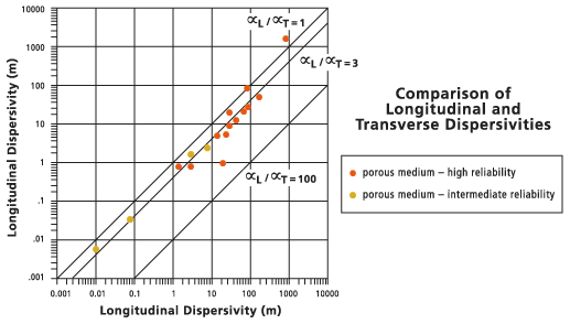
Similar caveats apply to the estimation of the ratio of longitudinal to transverse dispersivities presented in the following figure. These values are commonly related by a simple ratio, though again, you should experiment with a range of values.

The default dispersivity ratio  is indicated by the solid line (the center line) in the figure below. The dotted lines (the outer lines) are placed at
  and
and  for comparison.
Gelhar et al includes values for effective porosity and transmissivity in the tabulation. Tables for these values can be found in Freeze and Cherry (1979) and Marsily (1986).
Retardation
Retardation is the ratio between the velocity of the transporting fluid and that of the solute and is expressed as a number between one and infinity, with no units. A retardation of two means that the solute migrates through the porous medium at half the seepage velocity. An ideal tracer undergoes no adsorption and travels in the solution with the fluid. Such a solute has a retardation of one, meaning that it moves at the same rate as the transporting fluid.
This phenomenon is the result of adsorption and desorption of the constituent into the porous matrix, especially into organic coatings on the pore walls. The retardation equation is presented in a discussion by Freeze and Cherry (1979) as:

where:
 : The matrix bulk density.
n : The porosity of the formation.
Kd : The distribution coefficient, which represents the partitioning due to fast, reversible adsorption of a solute between liquid and solid phases assuming a linear isotherm.
Marsily (1986) also discusses the retardation factor and adsorption in detail.
Performing advection–dispersion modeling
The tools Darcy Flow, Particle Track, and Porous Puff can be used to perform rudimentary advection–dispersion modeling of constituents in groundwater. Darcy Flow generates a groundwater flow velocity field from geologic data, Particle Track follows the path of advection through the flow field from a point source, and Porous Puff calculates the hydrodynamic dispersion of an instantaneous point release of a constituent as it is advected along the flow path.
A complete discussion of advection–dispersion modeling using these tools is presented in Tauxe (1994).
The typical sequence for groundwater modeling is to perform Darcy Flow, then Particle Track, then Porous Puff.
Example
- An example of the tool dialog box for Porous Puff follows:
Input particle track file : ttrack.txt
Input effective formation porosity raster : poros
Input saturated thickness raster : thickn
Output raster : ppuff1
Mass : 3.2e7
Dispersion time : 50000
Longitudinal dispersivity : 6
Dispersivity ratio : 3
Retardation factor : 1
Decay coefficient : 250
- An example of using Porous Puff in Map Algebra is:
outPPuff1 = PorousPuff(ttrack.txt, poros, thickn, 1000000, 0.01, 10, 1.5, 1.0, 500)
- A sequence of Map Algebra expressions involving the suite of groundwater modeling
tools follows:
out_vol = DarcyFlow(head, poros, thickn, transm, dir1, mag1)
ParticleTrack(dir1, mag1, ttrack.txt, 500, 650, "#", "#", track_feat.shp)
out_puff = PorousPuff(ttrack.txt, poros, thickn, 3.2e7, 50000, 6, 3, 1, 250)
References
Bear, J. 1979, Hydraulics of Groundwater. McGraw–Hill.
Freeze, R. A., and J. A. Cherry. 1979. Groundwater. Prentice–Hall.
Gelhar, L. W., C. Welty, and K. R. Rehfeldt. 1992. "A Critical Review of Data on Field-Scale Dispersion in Aquifers". Water Resources Research 28 (7): 1955–1974.
Marsily, G. de. 1986. Quantitative Hydrogeology. Academic Press.
Tauxe, J. D. 1994. "Porous Medium Advection–Dispersion Modeling in a Geographic Information System". Ph.D. diss., University of Texas, Austin.