Output generated from the OLS Regression tool includes the following:
- Output feature class
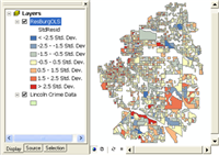
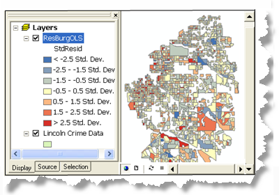
Map of OLS Residuals - Message window report of statistical results
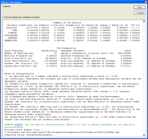
OLS Statistical Report - Optional PDF report file
- Optional table of explanatory variable coefficients

Coefficient table of OLS Model Results - Optional table of regression diagnostics

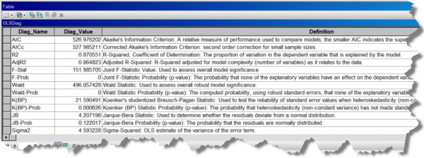
OLS Model Diagnostics Table
Each of these outputs is shown and described below as a series of steps for running OLS regression and interpreting OLS results.
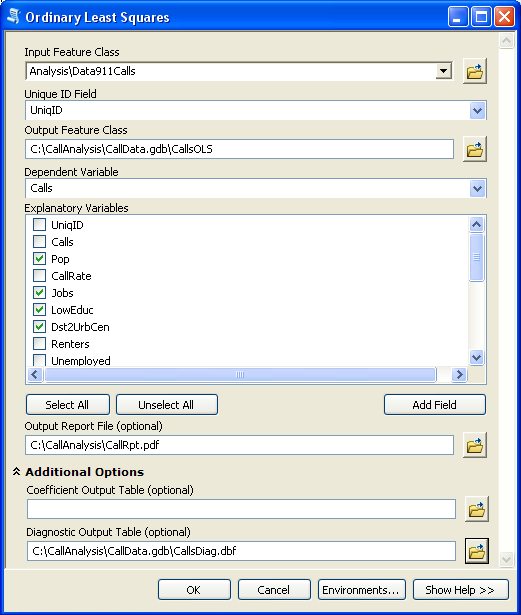
(A) To run the OLS tool, provide an Input Feature Class with a Unique ID Field, the Dependent Variable you want to model/explain/predict, and a list of Explanatory Variables. You will also need to provide a path for the Output Feature Class and, optionally, paths for the Output Report File, Coefficient Output Table, and Diagnostic Output Table.
After OLS runs, the first thing you will want to check is the OLS summary report, which is written as messages during tool execution and written to a report file when you provide a path for the Output Report File parameter.
(B) Examine the summary report using the numbered steps described below:
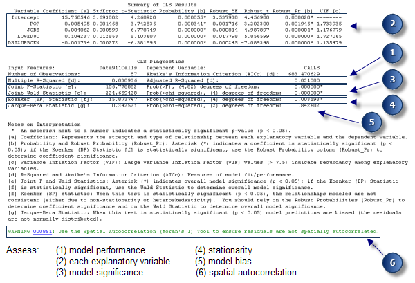
Dissecting the Statistical Report
- Assess model performance. Both the Multiple R-Squared and Adjusted R-Squared values are measures of model performance. Possible values range from 0.0 to 1.0. The Adjusted R-Squared value is always a bit lower than the Multiple R-Squared value, because it reflects model complexity (the number of variables) as it relates to the data and is consequently a more accurate measure of model performance. Adding an additional explanatory variable to the model will likely increase the Multiple R-Squared value but may decrease the Adjusted R-Squared value. Suppose you are creating a regression model of residential burglary (the number of residential burglaries associated with each census block is your dependent variable, y). An Adjusted R-Squared value of 0.39 would indicate that your model (your explanatory variables modeled using linear regression) explains approximately 39 percent of the variation in the dependent variable. Said another way, your model tells approximately 39 percent of the residential burglary story.

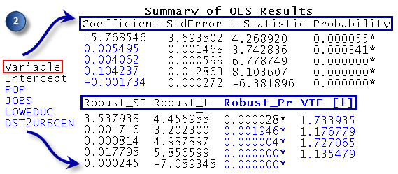
R-Squared Values Quantify Model Performance - Assess each explanatory variable in the model: Coefficient, Probability or Robust Probability, and Variance Inflation Factor (VIF). The coefficient for each explanatory variable reflects both the strength and type of relationship the explanatory variable has to the dependent variable. When the sign associated with the coefficient is negative, the relationship is negative (for example, the larger the distance from the urban core, the smaller the number of residential burglaries). When the sign is positive, the relationship is positive (for example, the larger the population, the larger the number of residential burglaries). Coefficients are given in the same units as their associated explanatory variables (a coefficient of 0.005 associated with a variable representing population counts may be interpreted as 0.005 people). The coefficient reflects the expected change in the dependent variable for every 1 unit change in the associated explanatory variable, holding all other variables constant (for example, a 0.005 increase in residential burglary is expected for each additional person in the census block, holding all other explanatory variables constant). The T test is used to assess whether or not an explanatory variable is statistically significant. The null hypothesis is that the coefficient is, for all intents and purposes, equal to zero (and consequently is not helping the model). When the probability or robust probability (p-value) is very small, the chance of the coefficient being essentially zero is also small. If the Koenker test (see below) is statistically significant, use the robust probabilities to assess explanatory variable statistical significance. Statistically significant probabilities have an asterisk (*) next to them. An explanatory variable associated with a statistically significant coefficient is important to the regression model if theory/common sense supports a valid relationship with the dependent variable, if the relationship being modeled is primarily linear, and if the variable is not redundant to any other explanatory variables in the model. The VIF measures redundancy among explanatory variables. As a rule of thumb, explanatory variables associated with VIF values larger than about 7.5 should be removed (one by one) from the regression model. If, for example, you have a population variable (the number of people) and an employment variable (the number of employed persons) in your regression model, you will likely find them to be associated with large VIF values indicating that both of these variables are telling the same story; one of them should be removed from your model.
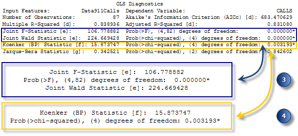
Assess which variables are statistically significant. - Assess model significance. Both the Joint F-Statistic and Joint Wald Statistic are measures of overall model statistical significance. The Joint F-Statistic is trustworthy only when the Koenker (BP) statistic (see below) is not statistically significant. If the Koenker (BP) statistic is significant, you should consult the Joint Wald Statistic to determine overall model significance. The null hypothesis for both of these tests is that the explanatory variables in the model are not effective. For a 95 percent confidence level, a p-value (probability) smaller than 0.05 indicates a statistically significant model.
Assess the overall statistical significance of the regression model. - Assess Stationarity. The Koenker (BP) Statistic (Koenker's studentized Bruesch-Pagan statistic) is a test to determine whether the explanatory variables in the model have a consistent relationship to the dependent variable both in geographic space and in data space. When the model is consistent in geographic space, the spatial processes represented by the explanatory variables behave the same everywhere in the study area (the processes are stationary). When the model is consistent in data space, the variation in the relationship between predicted values and each explanatory variable does not change with changes in explanatory variable magnitudes (there is no heteroscedasticity in the model). Suppose you want to predict crime, and one of your explanatory variables is income. The model would have problematic heteroscedasticity if the predictions were more accurate for locations with small median incomes than they were for locations with large median incomes. The null hypothesis for this test is that the model is stationary. For a 95 percent confidence level, a p-value (probability) smaller than 0.05 indicates statistically significant heteroscedasticity and/or nonstationarity. When results from this test are statistically significant, consult the robust coefficient standard errors and probabilities to assess the effectiveness of each explanatory variable. Regression models with statistically significant nonstationarity are often good candidates for Geographically Weighted Regression (GWR) analysis.
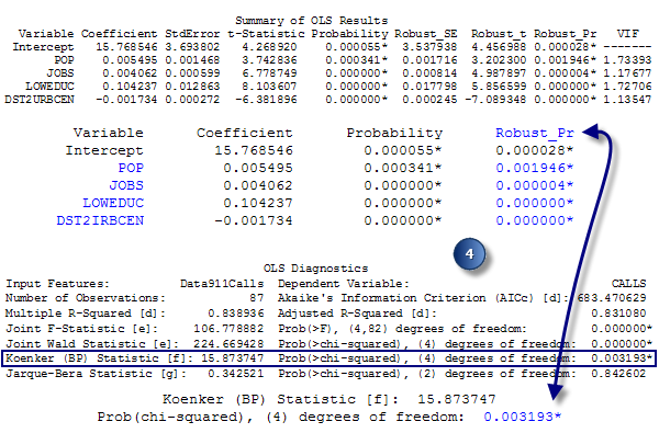
Assess stationarity: if the Koenker test is statistically significant (*), consult the robust probabilities to determine whether explanatory variable coefficients are significant or not. - Assess model bias. The Jarque-Bera statistic indicates whether or not the residuals (the observed/known dependent variable values minus the predicted/estimated values) are normally distributed. The null hypothesis for this test is that the residuals are normally distributed, so if you were to construct a histogram of those residuals, they would resemble the classic bell curve, or Gaussian distribution. When the p-value (probability) for this test is small (smaller than 0.05 for a 95 percent confidence level, for example), the residuals are not normally distributed, indicating your model is biased. If you also have statistically significant spatial autocorrelation of your residuals (see below), the bias may be the result of model misspecification (a key variable is missing from the model). Results from a misspecified OLS model are not trustworthy. A statistically significant Jarque-Bera test can also occur if you are trying to model nonlinear relationships, if your data include influential outliers, or when there is strong heteroscedasticity.

Assess model bias. - Assess residual spatial autocorrelation. Always run the Spatial Autocorrelation (Moran's I) tool on the regression residuals to ensure that they are spatially random. Statistically significant clustering of high and/or low residuals (model under- and overpredictions) indicates a key variable is missing from the model (misspecification). OLS results cannot be trusted when the model is misspecified.

Use the Spatial Autocorrelation tool to ensure that model residuals are not spatially autocorrelated. - Finally, review the section titled How Regression Models Go Bad in the Regression Analysis Basics document as a check that your OLS regression model is properly specified. If you are having trouble finding a properly specified regression model, the Exploratory Regression tool can be very helpful. The Notes on Interpretation at the end of the OLS summary report are there to help you remember the purpose of each statistical test and to guide you toward a solution when your model fails one or more of the diagnostics.
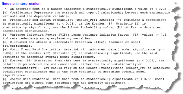
The OLS report includes Notes to help you interpret diagnostic output.
(C) If you provide a path for the optional Output Report File, a PDF will be created that contains all of the information in the summary report plus additional graphics to help you assess your model. The first page of the report provides information about each explanatory variable. Similar to the first section of the summary report (see number 2 above) you would use the information here to determine if the coefficients for each explanatory variable are statistically significant and have the expected sign (+/-). If the Koenker test is statistically significant (see number 4 above), you can only trust the robust probabilities to decide if a variable is helping your model or not. Statistically significant coefficients will have an asterisk next to their p-values for the probabilities and/or robust probabilities columns. You can also tell from the information on this page of the report whether any of your explanatory variables are redundant (exhibit problematic multicollinearity). Unless theory dictates otherwise, explanatory variables with elevated Variance Inflation Factor (VIF) values should be removed one by one until the VIF values for all remaining explanatory variables are below 7.5.

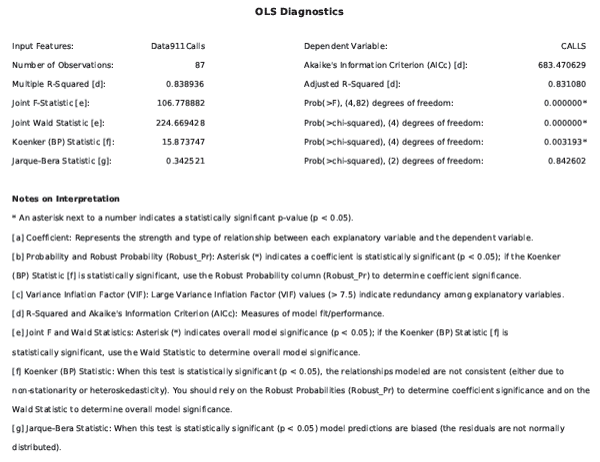
The next section in the Output Report File lists results from the OLS diagnostic checks. This page also includes Notes on Interpretation describing why each check is important. If your model fails one of these diagnostics, refer to the table of common regression problems outlining the severity of each problem and suggesting potential remediation. The graphs on the remaining pages of the report will also help you identify and remedy problems with your model.
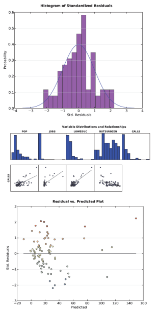
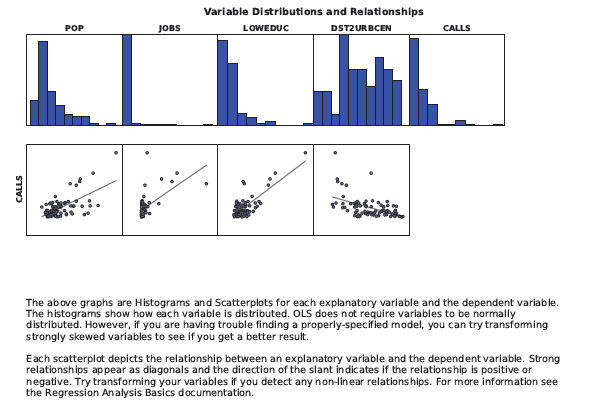
The third section of the Output Report File includes histograms showing the distribution of each variable in your model, and scatterplots showing the relationship between the dependent variable and each explanatory variable. If you are having trouble with model bias (indicated by a statistically significant Jarque-Bera p-value), look for skewed distributions among the histograms, and try transforming these variables to see if this eliminates bias and improves model performance. The scatterplots show you which variables are your best predictors. Use these scatterplots to also check for nonlinear relationships among your variables. In some cases, transforming one or more of the variables will fix nonlinear relationships and eliminate model bias. Outliers in the data can also result in a biased model. Check both the histograms and the scatterplots for these data values and/or data relationships. Try running the model with and without an outlier to see how much it is impacting your results. You may discover that the outlier is invalid data (entered or recorded in error) and be able to remove the associated feature from your dataset. If the outlier reflects valid data and is having a very strong impact on the results of your analysis, you may decide to report your results both with and without the outlier(s).
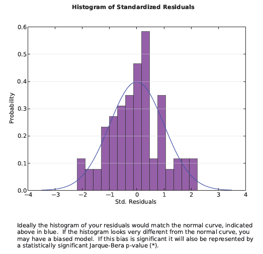
When you have a properly specified model, the over- and underpredictions will reflect random noise. If you were to create a histogram of random noise, it would be normally distributed (think bell curve). The fourth section of the Output Report File presents a histogram of the model over- and underpredictions. The bars of the histogram show the actual distribution, and the blue line superimposed on top of the histogram shows the shape the histogram would take if your residuals were, in fact, normally distributed. Perfection is unlikely, so you will want to check the Jarque-Bera test to determine if deviation from a normal distribution is statistically significant or not.
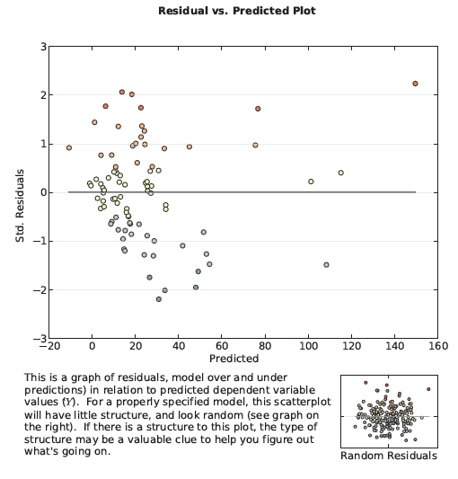
The Koenker diagnostic tells you if the relationships you are modeling either change across the study area (nonstationarity) or vary in relation to the magnitude of the variable you are trying to predict (heteroscedasticity). Geographically Weighted Regression will resolve issues with nonstationarity; the graph in section 5 of the Output Report File will show you if you have a problem with heteroscedasticity. This scatterplot graph (shown below) charts the relationship between model residuals and predicted values. Suppose you are modeling crime rates. If the graph reveals a cone shape with the point on the left and the widest spread on the right of the graph, it indicates your model is predicting well in locations with low rates of crime, but not doing well in locations with high rates of crime.
The last page of the report records all of the parameter settings that were used when the report was created.
(D) Examine the model residuals found in the Output Feature Class. Over- and underpredictions for a properly specified regression model will be randomly distributed. Clustering of over- and/or underpredictions is evidence that you are missing at least one key explanatory variable. Examine the patterns in your model residuals to see if they provide clues about what those missing variables might be. Sometimes running Hot Spot Analysis on regression residuals helps you identify broader patterns. Additional strategies for dealing with an improperly specified model are outlined in: What they don't tell you about regression analysis.
(E) View the coefficient and diagnostic tables. Creating the coefficient and diagnostic tables is optional. While you are in the process of finding an effective model, you may elect not to create these tables. The model-building process is iterative, and you will likely try a large number of different models (different explanatory variables) until you settle on a few good ones. You can use the Corrected Akaike Information Criterion (AICc) on the report to compare different models. The model with the smaller AICc value is the better model (that is, taking into account model complexity, the model with the smaller AICc provides a better fit with the observed data).

Creating the coefficient and diagnostic tables for your final OLS models captures important elements of the OLS report. The coefficient table includes the list of explanatory variables used in the model with their coefficients, standardized coefficients, standard errors, and probabilities. The coefficient is an estimate of how much the dependent variable would change given a 1 unit change in the associated explanatory variable. The units for the coefficients matches the explanatory variables. If, for example, you have an explanatory variable for total population, the coefficient units for that variable reflect people; if another explanatory variable is distance (meters) from the train station, the coefficient units reflect meters. When the coefficients are converted to standard deviations, they are called standardized coefficients. You can use standardized coefficients to compare the effect diverse explanatory variables have on the dependent variable. The explanatory variable with the largest standardized coefficient after you strip off the +/- sign (take the absolute value) has the largest effect on the dependent variable. Interpretations of coefficients, however, can only be made in light of the standard error. Standard errors indicate how likely you are to get the same coefficients if you could resample your data and recalibrate your model an infinite number of times. Large standard errors for a coefficient mean the resampling process would result in a wide range of possible coefficient values; small standard errors indicate the coefficient would be fairly consistent.

The diagnostic table includes results for each diagnostic test, along with guidelines for how to interpret those results.
Additional resources
There are a number of good resources to help you learn more about OLS regression on the Spatial Statistics Resources page. Start by reading the Regression Analysis Basics documentation and/or watching the free one-hour Esri Virtual CampusRegression Analysis Basics web seminar. Next, work through a Regression Analysis tutorial. Apply regression analysis to your own data, referring to the table of common problems and the article called What they don't tell you about regression analysis for additional strategies. If you are having trouble finding a properly specified model, the Exploratory Regression tool can be very helpful.