One of the most basic questions asked of a GIS is "What's on top of what?" For example:
- What land use is on top of what soil type?
- What parcels are within the 100-year floodplain? ("Within" is just another way of saying "on top of.")
- What roads are within what counties?
- What wells are within abandoned military bases?
To answer such questions before the days of GIS, cartographers would create maps on clear plastic sheets and overlay these sheets on a light table to create a new map of the overlaid data. Because overlay yields such valuable information, it was paramount to the development of GIS.
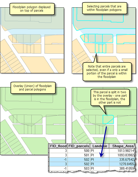
An overlay operation is much more than a simple merging of line work; all the attributes of the features taking part in the overlay are carried through, as shown in the example below, where parcels (polygons) and flood zones (polygons) are overlaid (using the Union tool) to create a new polygon dataset. The parcels are split where they are crossed by the flood zone boundary, and new polygons created. The FID_flood value indicates whether polygons are outside (-1) or inside the flood zone, and all polygons retain their original land-use category values.
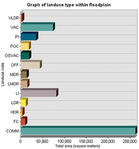
The total area of each land-use type in the flood zone can be calculated by selecting all polygons within the flood zone (using the Select Layer By Attribute tool, for example) and summarizing the area by land-use type (using the Frequency tool). Following is a chart illustrating the result of this calculation.
Similarly, you'd overlay watershed boundaries with a vegetation layer to calculate the amount of each vegetation type in each watershed.
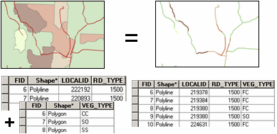
In the illustration below, logging roads (lines) and vegetation types (polygons) are overlaid to create a new line feature class. The lines have been split where they were intersected by polygons, and each line feature has been assigned the attributes of both original layers. The lines are shown symbolized by the vegetation type associated with each.
You can use overlay analysis to combine the characteristics of several datasets into one. You can then find specific locations or areas that have a certain set of attribute values—that is, match the criteria you specify. This approach is often used to find locations that are suitable for a particular use or are susceptible to some risk. For example, you'd overlay layers of vegetation type, slope, aspect, soil moisture, and so on, to find areas susceptible to wildfire.
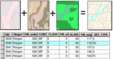
Below is an example of an overlay of steep slopes, soils, and vegetation. New polygons are created by the intersection of the input polygon boundaries. The resulting polygons have all the attributes of the original polygons.
Overlay analysis is often used in conjunction with other types of analysis. For example, you might include datasets derived from proximity analysis (such as the Buffer tool) or surface analysis (the Slope or Aspect tool). Similarly, you'll likely perform additional analysis on the results of the overlay, such as extraction to select a subset of features, or generalization (to dissolve polygons, for example). Often, overlay is one step in an analysis process or model and may occur at various points in the process.
Overlay methods
In general, there are two methods for performing overlay analysis—feature overlay (overlaying points, lines, or polygons) and raster overlay. Some types of overlay analysis lend themselves to one or the other of these methods. Overlay analysis to find locations meeting certain criteria is often best done using raster overlay (although you can do it with feature data). Of course, this also depends on whether your data is already stored as features or rasters. It may be worthwhile to convert the data from one format to the other to perform the analysis.
Feature overlay
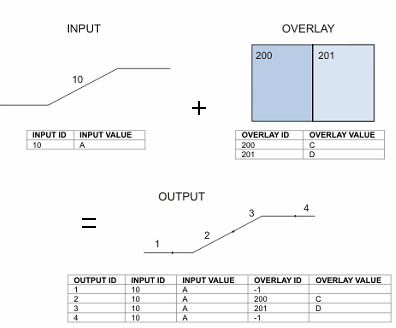
The key elements in feature overlay are the input layer, the overlay layer, and the output layer. The overlay function splits features in the input layer where they are overlapped by features in the overlay layer. New areas are created where polygons intersect. If the input layer contains lines, the lines are split where polygons cross them. These new features are stored in the output layer—the original input layer is not modified. The attributes of features in the overlay layer are assigned to the appropriate new features in the output layer, along with the original attributes from the input layer.
Below is an example of line-on-polygon overlay. The line is split at the polygon boundaries, and each of the resulting line features has the original line attributes plus the attributes of the polygon it fell within.
Raster overlay
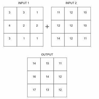
In raster overlay, each cell of each layer references the same geographic location. That makes it well suited to combining characteristics for numerous layers into a single layer. Usually, numeric values are assigned to each characteristic, allowing you to mathematically combine the layers and assign a new value to each cell in the output layer.
Below is an example of raster overlay by addition. Two input rasters are added together to create an output raster with the values for each cell summed.
This approach is often used to rank attribute values by suitability or risk, then add them to produce an overall rank for each cell. The various layers can also be assigned a relative importance to create a weighted ranking (the ranks in each layer are multiplied by that layer's weight value before being summed with the other layers).
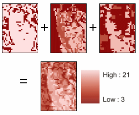
Below is an example of raster overlay by addition for suitability modeling. Three raster layers (steep slopes, soils, and vegetation) are ranked for development suitability on a scale of 1 to 7. When the layers are added (bottom), each cell is ranked on a scale of 3 to 21.
Alternatively, you can assign a value to each cell in the output layer based on unique combinations of values from several input layers.
Overlay tools
Vector overlay tools
Feature overlay tools are located in the Analysis toolbox in the Overlay toolset. Conceptually, the tools are similar—they differ by the feature types they allow you to overlay, by whether you can overlay multiple layers at one time, and by which input and overlay features are maintained in the output layer.
| Tool | Binary or multiple overlay | Input data type | Overlay data type | Output |
|---|---|---|---|---|
Binary | Any | Polygon or same as input | Input features, split by overlay features | |
Multiple | Any | N/A | Only features common to all input layers | |
Binary | Any | Same as input | Features common to either input layer or overlay layer but not both | |
Multiple | Polygon | N/A | All input features | |
Binary | Any | Polygon | Input feature geometry replaced by update layer |
The table below shows the results of overlaying an input dataset and an overlay dataset using each tool.
| Input features | Overlay features | Operation | Result |
|---|---|---|---|
|
|
| |
|
|
| |
|
|
| |
|
|
| |
|
|
|
Raster overlay tools
Raster overlay tools are located in several toolsets in the Spatial Analyst toolbox. Spatial Analyst is an ArcGIS extension that is licensed separately. If your site has a Spatial Analyst license and the Spatial Analyst extension has been installed, you will have access to the Spatial Analyst toolbox in ArcToolbox.
| Tool | Location | What it does |
|---|---|---|
Summarizes values in a raster layer by zones (categories) in another layer—for example, calculate the mean elevation for each vegetation category. | ||
Assigns a value to each cell in the output layer based on unique combinations of values from several input layers. | ||
Automates the raster overlay process and lets you assign weights to each layer before adding (you can also specify equal influence to create an unweighted overlay). | ||
Overlays several rasters, multiplying each by their given weight and summing them together. |


