Inherent in GIS data is information on the attributes of features as well as their locations. This information is used to create maps that can be visually analyzed. Statistical analysis helps you extract additional information from your GIS data that might not be obvious simply by looking at a map—information such as how attribute values are distributed, whether there are spatial trends in the data, or whether the features form spatial patterns. Unlike query functions—such as identify or selection, which provide information about individual features—statistical analysis reveals the characteristics of a set of features as a whole.
Some of the statistical analysis techniques described in this document are most well-suited for interactive applications, such as ArcMap, that allow you to select and visualize data in an ad-hoc and fluid environment. Some of the methods described here are found in ArcMap's menus and toolbars and don't have a geoprocessing tool counterpart. Other methods, such as the spatial statistics tools, are only implemented as geoprocessing tools.
Uses of statistical analysis
Statistical analysis is often used to explore your data—for example, to examine the distribution of values for a particular attribute or to spot outliers (extreme high or low values). Having this information is useful when defining classes and ranges on a map, when reclassifying data, or when looking for data errors.
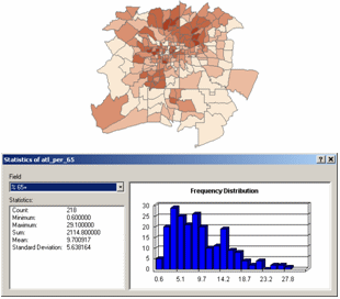
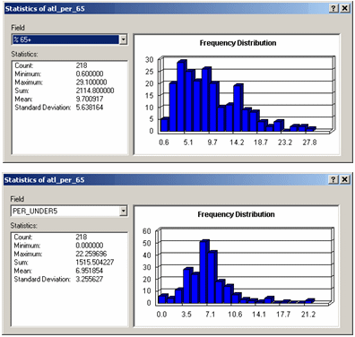
In the example below, statistics have been calculated for the distribution of senior citizens by census tract in this region (percentage of those aged 65 and over in each tract), including the mean and standard deviation, as well as a histogram showing the distribution of values. Most tracts have a lower percentage of seniors than the mean, but a few tracts have a very high percentage.
Another use of statistical analysis is to summarize data. Often, this is done for categories, such as calculating the total area in each land-use category. You can also create spatial summaries, such as calculating the average elevation for each watershed. Summary data is useful for gaining a better understanding of conditions in a study area.
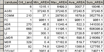
In the example below, summary statistics have been calculated for each land-use class showing the number of parcels in that class, the size of the smallest and largest parcel, the average parcel size, and the total area in the class.
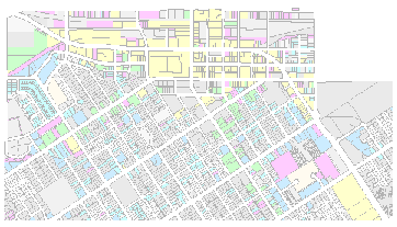
Statistical analysis is also used to identify and confirm spatial patterns, such as the center of a group of features, the directional trend, or whether features form clusters. While patterns may be apparent on a map, trying to draw conclusions from a map can be difficult—how you classify and symbolize the data can obscure or overemphasize patterns. Statistical functions analyze the underlying data and give you a measure that can be used to confirm the existence and strength of the pattern.
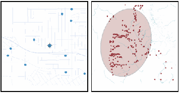
Below is an example of analyses that show the mean center of a set of burglaries, and the standard deviation ellipse for a set of moose sightings (showing the directional trend).
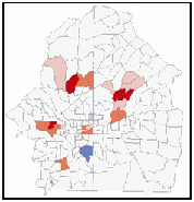
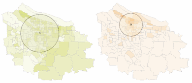
Below is an example of an analysis that shows statistically significant clusters of census tracts with many senior citizens (orange) or few (blue).
Types of statistical analysis
Statistical analysis functions in ArcGIS for Desktop are either nonspatial (tabular) or spatial (containing location).
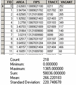
Nonspatial statistics are used to analyze attribute values associated with features. The values are accessed directly from a layer's feature attribute table. Examples of nonspatial statistics include the mean and standard deviation.
In this example, the Summary Statistics tool was used to calculate the number of vacant parcels for a set of census tracts, including the total, the mean, and the standard deviation.
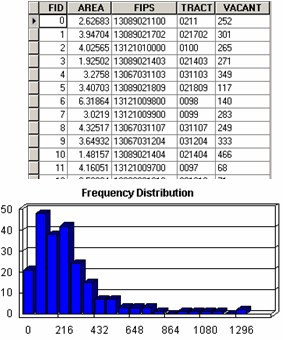
Charts and graphs, such as a histogram or Q-Q plots, are another way of analyzing nonspatial data. In all cases, only the values are analyzed. The locations of the features with which the values are associated—and any spatial relationships between the features—are not considered.
In this example, the histogram shows the distribution of vacant parcels (the number of vacant parcels along the x-axis and the number of tracts in each range along the y-axis).
A Normal Q-Q Plot is used to assess the similarity of the distribution of a set of values to that of a standard normal distribution (the typical bell curve, when shown on a histogram). The line on the Normal Q-Q plot shows expected values for a normal distribution—the closer the values to the line, the closer the distribution is to normal. In this example, the concentration of the elements Phosphorous for a set of soil samples is close to normally distributed.
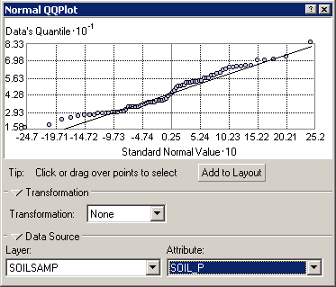
The Normal QQ Plot tool is one of the data exploration tools available with the Geostatistical Analyst extension.
Spatial statistics, on the other hand, focus on the spatial relationships between features—how compact or dispersed the features are, whether they're oriented in a particular direction, and whether they form clusters. The spatial relationship is usually defined as distance (how far apart features are) but can also be other forms of interaction between features.
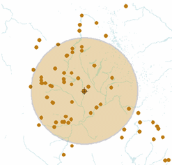
In the example below, the output of the Standard Distance tool (displayed graphically as a circle) is calculated using the distance of each wildlife sighting from the calculated center of the sightings.
Some spatial statistics consider both the spatial relationships of features and the values of an attribute associated with the features. These are known as weighted statistics—the spatial relationship is influenced by the values. Weighted spatial statistics are used to find out if features having similar values occur together—if, for example, schools with similarly high or low test scores form clusters.
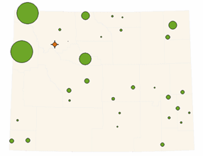
In the example below, the center of parks is weighted by the number of visitors at each park (represented by the size of the green circles).
Statistical functions can also be classified by whether they're descriptive or inferential. Descriptive statistics summarize some characteristic of the values or features you're analyzing—the mean value, the frequency distribution of values, or the directional trend of a group of features. Descriptive statistics are often useful for comparing two sets of features for the same area.
The example below compares the distribution of senior citizens (top) to that of children under 5 (bottom) for the same set of census tracts.
In the example below, the standard distance circles for the American Indian and African American population show that the distribution of the African American population in this area is much more compact.
Inferential statistics use probability theory to either predict the likely occurrence of values (using a set of known values), or to assess the likelihood that any pattern or trend you see in the data is not due to chance. The function provides a measure of the pattern or relationship. You then perform a statistical test on this measure to determine whether it is significant at some level of confidence. If the statistic analysis indicates that burglaries occur in clusters, you'd then run a test to find out the chance that the clusters occurred by chance. You might find, for example, that there's a 90 percent likelihood that the clusters didn't occur by chance, indicating the burglaries may be linked in some way. Essentially to determine the probability, the test compares the measure you get for the existing features to the measure you'd expect to get for the same number of features spread over the same area, but distributed randomly.
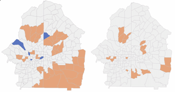
In the example below, the map on the left shows clusters of census tracts having a high number of senior citizens (orange) or a low number (blue), at a 90 percent level of probability; the right map shows clusters at a 99 percent level of probability.
Statistical analysis functions
The statistical functions in ArcGIS for Desktop are located in ArcMap, ArcCatalog, and geoprocessing, as well as within two extensions: Spatial Analyst and Geostatistical Analyst.
Table statistics
A core set of descriptive statistics that summarize the values for a single field is available from several locations in ArcGIS for Desktop—the table window in ArcMap, the table preview tab in ArcCatalog, and the Statistics toolset (within the Analysis toolbox).
| Function | Location | Statistics | Output |
|---|---|---|---|
Statistics menu option | ArcMap table window or ArcCatalog table preview tab | Count, Minimum, Maximum, Sum, Mean, Standard Deviation, Frequency histogram | Results are displayed in a window. |
Summary Statistics tool | Minimum, Maximum, Sum, Mean, Standard Deviation, Range, First, Last | Results are written to a new table. |
To summarize a field by one or more other fields (for example, to count the number of parcels in each land-use class, sum the area in each land-use class, or find the average parcel size in each class), use the Summarize option on the ArcMap table window or the Frequency tool in the Statistics toolset in the Analysis toolbox.
| Function | Location | Statistics | Output |
|---|---|---|---|
Summarize menu option | ArcMap table window (right-click field name) | Minimum, Maximum, Average (mean), Sum, Standard Deviation, Variance | Results are written to a new table. |
Frequency tool | Count, Sum | Results are written to a new table. |
Spatial Statistics
The Spatial Statistics toolbox contains a number of statistical routines for analyzing the distribution of a set of features, analyzing patterns, and identifying clusters.
| Functional Area | Toolset | Tools |
|---|---|---|
Geographic distribution measurements | Mean Center, Central Feature, Standard Distance, Directional Distribution (Standard Deviational Ellipse), Linear Directional Mean | |
Geographic pattern analysis | Average Nearest Neighbor, Spatial Autocorrelation (Moran's I), High/Low Clustering (Getis-Ord General G) | |
Geographic cluster analysis | Cluster and Outlier Analysis (Anselin Local Moran's I), Hot Spot Analysis (Getis-Ord Gi*) | |
Regression analysis | Ordinary Least Squares, Exploratory Regression, Geographically Weighted Regression |
Raster statistics
The Spatial Analyst includes several statistical functions that can be used to analyze rasters, primarily to summarize attribute values and assign the summary statistics to cells in a new raster layer. These are located in several different toolsets with the Spatial Analyst toolbox.
| Tool | Location | Input | Output | What it does |
|---|---|---|---|---|
Multiple rasters | Raster | Calculates the specified statistic for each cell based on multiple inputs | ||
Raster | Raster | Summarizes the values for a raster within a defined neighborhood around each cell and assigns the value to that cell in the output raster | ||
Point features | Raster | Summarizes values for point feature attributes within a defined neighborhood and assigns values to cells in the output raster | ||
Line features | Raster | Summarizes values for line feature attributes within a defined neighborhood and assigns values to cells in the output raster | ||
Raster or polygon features | Raster or summary table | Summarizes values of a raster surface by categories or classes (zones) of the input raster or polygon dataset |
Data exploration tools
The Geostatistical Analyst—while focusing on the creation of surface from a set of sample points—also contains a set of tools for visual exploration of data values using charts and graphs. These are often used prior to surface creation to decide which parameters to use for a specific set of data but can also be used generally to explore your dataset. The tools allow you to explore the distribution of values, whether there is a directional trend in the data, and whether there are relationships between two attributes (for example, to see if the values vary together or inversely). The tools are available from the Explore Data option on the Geostatistical Analyst toolbar.