Comparing models

Available with Geostatistical Analyst license.

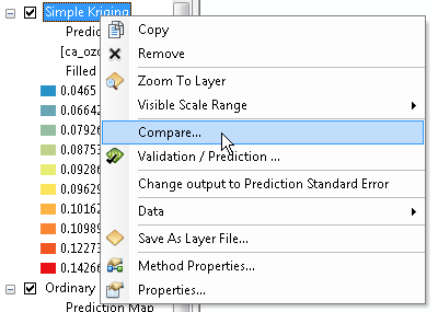
Comparison helps you determine how good the model that created a geostatistical layer is relative to another model. To compare models, you must have two geostatistical layers for comparison (created using the ArcGIS Geostatistical Analyst extension). These two layers may have been created using different interpolation methods (for example, IDW and ordinary kriging) or by using the same method with different parameters. In the first case, you are comparing which method is best for your data, and in the second, you are examining the effects of different input parameters on a model when creating the output surface. To compare two models, right-click on one of their names in the table of contents and click Compare, as shown below:

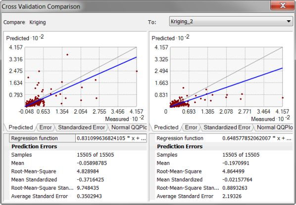
The Comparison dialog box uses the cross-validation statistics discussed in Performing cross-validation and validation. However, it allows you to examine the statistics and the plots side by side. Generally, the best model is the one that has the standardized mean nearest to zero, the smallest root-mean-squared prediction error, the average standard error nearest the root-mean-squared prediction error, and the standardized root-mean-squared prediction error nearest to 1.

It is common practice to create many surfaces before one is identified as best and will be final in itself or will be passed into a larger model (for example, a suitability model for siting houses) to solve an existing problem. You can systematically compare each surface with another, eliminating the worst of the two being compared, until the two best surfaces remain and are compared with one another. You can conclude that for this particular analysis, the best of the final two surfaces is the best surface possible.

Concerns when comparing methods and models

There are two issues to consider when comparing the results from different methods and/or models: one is optimality and the other is validity.

For example, the root-mean-squared prediction error may be smaller for a particular model. Therefore, you might conclude that it is the optimal model. However, when comparing to another model, the root-mean-squared prediction error may be closer to the average estimated prediction standard error. This is a more valid model, because when you predict at a point without data, you have only the estimated standard errors to assess your uncertainty of that prediction. You also must check that the root-mean-square standardized is close to one. When the root-mean-square standardized is close to one and the average estimated prediction standard errors are close to the root-mean-squared prediction errors from cross-validation, you can be confident that the model is appropriate. In the figure above, the kriging model on the left has a lower root-mean-square and a lower average standard error than the model on the right, but the kriging model on the right should be preferred because the root-mean-square and the average standard error are closer. Additionally, the model on the left has a very large root-mean-square standardized, which indicates severe model problems.

In addition to the statistics provided on the Comparison dialog box, you should use prior information that you have on the dataset and that you derived in ESDA when evaluating which model is best.

1. Right-click one of the geostatistical layers you want to compare in the ArcMap table of contents and click Compare.
2. Click the second layer in the comparison in the To drop-down menu.
3. Click the various tabs to see the different results of the comparison.
4. Click Close.