Available with Spatial Analyst license.
Within the cost distance and the path distance tools, defining the source characteristics of the mover allows control over the following:
- Different modes of travel from the different sources (for example, traveling by car or walking)
- Magnitudes at the sources (for example, different number of military troops at each location)
- A cost decay function (for example, a hiker gets fatigued)
- The starting cost from a source (for example, the time it takes to get the truck on the road)
- The capacities for sources (for example, how far a vehicle can travel before running out of fuel)
Some example problems solved by the source characteristics
Through the source characteristics you can address the following additional cost- and path-distance applications:
- Determine the area that can be searched for a lost hiker from two headquarters that have different modes of travel—ATVs at one and walking from the other.
- Explore the locations firefighters can reach from three facilities, accounting for the different number of firefighters based at each facility. There are 25 firefighters at the first facility, 15 at the second, and 10 at the third.
- Identify the best locations for campgrounds considering the energy loss of a hiker as they get tired.
- Analyze the time it will take to reach a remote brush fire while accounting for the 16 minutes it takes the firefighters to load their equipment.
- Define where to place refueling stations for tanks that need to travel a long distance to reach a distant objective in a military operation.
Cost distance formulas accounting for source characteristics
The cost distance formulas used to account for the source characteristics are detailed in the following sections.
Base cost distance formulas
There are two basic cost distance formulas that may apply, depending on how the adjacent cells are traversed.
Perpendicular cells
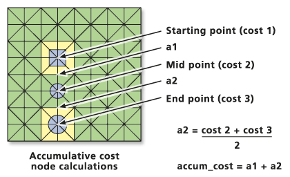
The cost distance formula to perpendicular cells is the following:
accum_cost = a1 + (cost2 + cost3)/2- Where
a1—The accumulative cost from cell 1 to cell 2
cost2—The cost of travel for cell 2
cost3—The cost of travel for cell 3
accum_cost—The accumulative cost to move into cell 3 from cell 1

Diagonal cells
The cost distance formula to diagonal cells is the following:
accum_cost = a1 + (1.4142 * ((cost2 + cost3)/2))Path distance formulas
There are two basic path distance formulas that may apply, depending on how the adjacent cells are traversed.
Perpendicular cells
accum_cost = a1 + ((((cost2 * HF(2)) + (cost3 * HF(3)))/2) * Surface_distance(23) * VF(23))Where
cost2—The cost of travel for cell 2
cost3 —The cost of travel for cell 3
HF(2)—The Horizontal factor for cell 2
HF(3)—The Horizontal factor for cell 3
Surface_distance(23)—The surface distance from 2 to 3
VF(23)—The Vertical factor from 2 to 3
Diagonal cells
accum_cost = a1 + ((((cost2 * HF(2)) + (cost3 * HF(3)))/2) * 1.414214 * Surface_distance(23) * VF(23))Cost and path distance formulas accounting for source characteristics
To account for the characteristics of the mover from the sources, the following formulas are applied.
Cost distance to perpendicular cells
accum_cost = (a1 * (1.0 + resistance_rate) + (((cost2 + cost3) / 2) * cost_multiplier))Where
resistance_rate—A dynamic adjustment to the accumulative cost to simulate a changing response to overcome the cost units as the accumulative cost increases, such as a hiker getting tired.
cost_multiplier—A multiplier to the cost units. The greater the value, the more costly the movement, such as walking versus riding an ATV.
Path distance to perpendicular cells
accum_cost = (a1 * (1 + resistance_rate)) + ((((cost2 * HF(2)) + (cost3 * HF(3)))/2)
              * Surface_distance(23) * VF(23) * cost_multiplier)
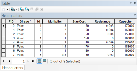
The source characteristics are identified by either a single value, which is applied to all the sources, or through a field in the attribute table associated with the sources, with each value being applied to the corresponding source.

Cost multiplier
Use case: Different modes of travel from each source—ATV versus walking.
Use case: Different magnitude of resources at each source—different number of firefighters at each headquarter.
Different modes of travel or different magnitudes at a source allow for an increase or decrease in movement speed or coverage over the cost surface. These characteristics increase or decrease the cost of movement through a cell.
The mode or magnitude can be implemented through the cost multiplier. ATVs would have a lower multiplier relative to walking since ATVs can overcome costs at a faster rate, while more firefighters based at a source can have a lower multiplier relative to a source with fewer firefighters since they can cover more area (can overcome the cost faster).
If the multiplier is a single value, it will be applied to all sources. If the modes or magnitudes (the multiplier) vary by source, the multiplier can be specified through a field associated with the sources.
Starting cost
Use case: Time it takes to prepare before leaving the source.
A starting cost can be identified by a single value, which will be added to each of the sources, or through a field associated with the sources, if the starting costs vary for the different sources. These are the fixed costs associated with the sources.
To reach the first cell, instead of starting the source calculations at zero using the following:
a1 = (((cost1 + cost2) / 2) * cost_multiplier)The accumulative formula is used with starting_cost, being the starting cost associated with the source:
a1 = starting_cost + (((cost1 + cost2) / 2) * cost_multiplier)Resistance rate
Use case: I am a hiker losing energy.
This is the only dynamically changing source characteristic. As the accumulative cost increases, so does the effect of the resistance rate. When determining the cost to move into a subsequent cell, conceptually, the accumulative cost to reach the cell is multiplied by the resistance rate, and the product is added to the running accumulative cost calculation. As a result, the effect of the rate is compounded with the traveler; therefore, the greater the resistance rate, the greater the effort it takes to overcome each subsequent cost unit—the traveler gets tired more quickly.
Since the resistance rate is similar to a compound rate, and generally the accumulative cost values are very large, small resistance rates are suggested (for example, 0.005).
Capacity
Use case: Identify potential locations for refueling stations for military tanks.
A cost capacity is defined for each source (or the modes of travel from the source), either by a single value or by a field. The dynamic cost distance algorithm continues to grow until the capacity for each source is reached. The output cost allocation can be different if the capacity parameter is set, as opposed to if it is not. That is, if a region with a low capacity is near a region with a high capacity, the high capacity region can capture some of the cells of the lower capacity region's original allocation when no capacity was set (but only those cells that have an accumulative cost greater than the defined capacity for the region with the lower capacity).