Available with Spatial Analyst license.
Segmentation and classification tools provide an approach to extracting features from imagery based on objects. These objects are created via an image segmentation process where pixels in close proximity and having similar spectral characteristics are grouped together into a segment. Segments exhibiting certain shapes, spectral, and spatial characteristics can be further grouped into objects. The objects can then be grouped into classes that represent real-world features on the ground. Image classification can also be performed on pixel imagery, for example, traditional unsegmented imagery.
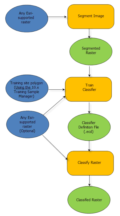
The object-oriented feature extraction process is a workflow supported by tools covering three main functional areas: image segmentation, deriving analytical information about the segments, and classification. Data output from one tool is the input to subsequent tools, where the goal is to produce a meaningful object-oriented feature class map. The object-oriented process is similar to a traditional image, pixel-based classification process, utilizing supervised and unsupervised classification techniques. Instead of classifying pixels, the process classifies segments, which can be thought of as super pixels. Each segment, or super pixel, is represented by a set of attributes that are used by the classifier tools to produce the classified image.
Below is a geoprocessing model that shows the object-oriented feature extraction workflow.

Image segmentation
The image segmentation is based on the Mean Shift approach. The technique uses a moving window that calculates an average pixel value to determine which pixels should be included in each segment. As the window moves over the image, it iteratively recomputes the value to make sure that each segment is suitable. The result is a grouping of image pixels into a segment characterized by an average color.
The Segment Mean Shift tool accepts any Esri-supported raster and outputs a 3-band, 8-bit color segmented image with a key property set to Segmented. The characteristics of the image segments depend on three parameters: spectral detail, spatial detail, and minimum segment size. You can vary the amount of detail that characterizes a feature of interest. For example, if you are more interested in impervious features than in individual buildings, adjust the spatial detail parameter to a small number; a lower number results in more smoothing and less detail.
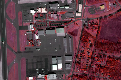
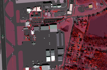
The image below is a segmented WorldView-2 scene, courtesy of DigitalGlobe, in color infrared. The segmented image shows similar areas grouped together without much speckle. It generalizes the area to keep all the features as a larger continuous area, rather than a more traditional classification that may have lots of random pixels scattered throughout the image.


References:
- D. Comanicu, P. Meer: Mean shift: A robust approach toward feature space analysis. IEEE Transactions on Pattern Analysis and Machine Intelligence, vol. 24, no. 5, May 2002.
- P. Meer, B. Georgescu: Edge detection with embedded confidence. IEEE Transactions on Pattern Analysis and Machine Intelligence, vol. 23, no. 12, December 2001.
- C. Christoudias, B. Georgescu, P. Meer: Synergism in low level vision. 16th International Conference of Pattern Recognition, Track 1 - Computer Vision and Robotics, Quebec City, Canada, August 2001.
Training sample data
Collecting training sample data means delineating a group of pixels representing particular features, which are delineated from the image. Then all the pixels in the image are statistically compared to the class definition that you specified and assigned to a particular feature class. Pixels that do not belong to any defined class are undefined. Training samples should not contain any unwanted pixels that do not belong to the class of interest. When you only choose the correct pixels for each class, the results often are characterized by a normal bell-shaped distribution. Make sure that your training sample polygon usually contains a significant number of pixels. For example, a 10 by 10 block of pixels equals 100 pixels, which is a reasonable size for a training polygon and is statistically significant.
A segmented raster dataset is different from a pixel image, in that each segment (sometimes referred to as a super pixel) is represented by one average color value. While it is easy to obtain a training sample polygon containing 100 pixels from an image, it is much more work to obtain 100 super pixels from a segmented raster dataset.
Parametric classifiers, such as the maximum likelihood classifier, needs a statistically significant number of samples to produce a meaningful probability density function. To achieve samples that are statistically significant, you should have 20 or more samples per class. This means each class, such as bare soil, deciduous trees, or asphalt, should have at least 20 segments collected to define each feature class.
Smoothing will affect the size and homogeneity of a segment. A segmented raster that used a high smoothing factor will likely contain segments that are large and contain multiple types of features visible in the source image. Due to the smoothing effect, it is recommended that training samples be collected on the segmented raster dataset. This will help ensure that training samples are collected from separate discrete segments.
Analytical information
The analytical information associated with the segmented layer is calculated by the classifier training tool and depends on the type of classifier specified. Use the appropriate training tool to classify your data:
| Classifier | Description |
|---|---|
| Train ISO Cluster Classifier | Generate an Esri classifier definition (.ecd) file using the Iso Cluster classification definition. |
| Train Maximum Likelihood Classifier | Generate an Esri classifier definition (.ecd) file using the Maximum Likelihood Classifier (MLC) classification definition. |
| Train Support Vector Machine Classifier | Generate an Esri classifier definition (.ecd) file using the Support Vector Machine (SVM) classification definition. The SVM classifier provides a powerful, modern supervised classification method that is able to handle a segmented raster input, or a standard image. This is a relatively new classification method that is widely used among researchers. |
The training tools ingest the image to be classified, an optional segmented layer, and training site polygon data to generate the appropriate Classifier Definition file. The training site file is generated from the existing Classificationtoolbar using the Training Sample Manager . The standard training sample file is used in the supervised classifiers.
The classifier definition .ecd file is based on the classifier specified and attributes of interest so that the classifier definition file is unique for each classifier, raster inputs, and attributes. It is similar to a classification signature file but is more general, in that it will support any classifier, and the generated classifier definition file is tailored for a specific combination of source data and classifier.
The classifier definition file can be based on any raster, not just segmented rasters. For example, a segmented raster is derived from IKONOS multispectral data, and the statistics and analytical attribute data can be generated from a 6-band, pan-sharpened WorldView-2 image, QuickBird, GeoEye, Pleiades, RapidEye, or Landsat 8 image. This flexibility allows you to derive the segmented raster once and generate classifier definition files and resulting classified feature maps using a multitude of image sources depending on your application.
Compute Segment Attributes
The tools outlined above are the most common tools utilized in the object-oriented workflow. An additional tool, Compute Segment Attributes, supports ingest and export of segmented rasters, both from and to third-party applications. This tool ingests a segmented image, a training site file, and an optional second raster to compute the attributes of each segment and outputs this information as an index raster file with associated attribute table.
The purpose of this tool is to allow for further analysis of the segmented raster. The attributes can be analyzed in a third-party statistics or graphics application or used as input to additional classifiers not supported by Esri. This tool also supports the ingest of a segmented raster from a third-party package and thus extends Esri capabilities, providing flexibility to utilize third-party data and applications packages.
Classification
The Classify Raster tool performs an image classification as specified by the Esri classifier definition file. Inputs to the tool include the image to be classified, the optional segmented raster (another raster dataset or a layer, such as a DEM), and a classifier definition file to generate the classified raster dataset. Note that the Classify Raster tool contains all the supported classifiers. The proper classifier is utilized depending on the properties and information contained in the classifier definition file. So the classifier definition file generated by the Train ISO Cluster Classifier, Train Maximum Likelihood Classifier, or Train Support Vector Machine Classifier tool will activate the corresponding classifier when you run Classify Raster.
Accuracy assessment
Accuracy assessment is an important part of any classification project; it compares the classified image to another data source considered to be accurate, or ground truth data. Ground truth can be collected in the field; however, this is time consuming and costly. Ground truth data can also be derived from interpreting high-resolution imagery, existing classified imagery, or GIS data layers.
The most common way to assess the accuracy of a classified map is to create a set of random points from the ground truth data and compare that to the classified data in a confusion matrix. Although this is a two-step process, you may need to compare the results of different classification methods or training sites, or you may not have ground truth data and are relying on the same imagery you used to create the classification. To accommodate these other workflows, the two-step process for accuracy assessment applies the following tools: Create Accuracy Assessment Points, Update Accuracy Assessment Points, and Compute Confusion Matrix.