The High/Low Clustering tool measures the concentration of high or low values for a given study area.
Calculations

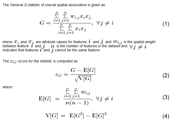
View additional General G statistic computations.
Notice that the only difference between the numerator and the denominator is the weighting (wij). High/Low Clustering will only work with positive values. Consequently, if your weights are binary (0/1) or are always less than 1, the range for General G will be between 0 and 1. A binary weighting scheme is recommended for this statistic. Select Fixed Distance Band, Polygon Contiguity, K Nearest Neighbors, or Delaunay Triangulation for the Conceptualization of Spatial Relationships parameter. Select None for the Standardization parameter.
Interpretation
The High/Low Clustering (Getis-Ord General G) tool is an inferential statistic, which means that the results of the analysis are interpreted within the context of the null hypothesis. The null hypothesis for the High/Low Clustering (General G) statistic states that there is no spatial clustering of feature values. When the p-value returned by this tool is small and statistically significant, the null hypothesis can be rejected (see What is a z-score? What is a p-value?). If the null hypothesis is rejected, then the sign of the z-score becomes important. If the z-score value is positive, the observed General G index is larger than the expected General G index, indicating high values for the attribute are clustered in the study area. If the z-score value is negative, the observed General G index is smaller than the expected index, indicating that low values are clustered in the study area.
The High/Low Clustering (Getis-Ord General G) tool is most appropriate when you have a fairly even distribution of values and are looking for unexpected spatial spikes of high values. Unfortunately, when both the high and low values cluster, they tend to cancel each other out. If you are interested in measuring spatial clustering when both the high values and the low values cluster, use the Spatial Autocorrelation tool.
The null hypothesis for both the High/Low Clustering (Getis-Ord General G) and the Spatial Autocorrelation (Global Moran's I) tool is complete spatial randomness (CSR); values are randomly distributed among the features in the dataset, reflecting random spatial processes at work. However, the interpretation of z-scores for the High/Low Clustering tool is very different from the interpretation of z-scores for the Spatial Autocorrelation (Global Moran's I) tool:
| Result | High/Low Clustering | Spatial Autocorrelation |
|---|---|---|
The p-value is not statistically significant. | You cannot reject the null hypothesis. It is quite possible that the spatial distribution of feature attribute values is the result of random spatial processes. Said another way, the observed spatial pattern of values could well be one of many, many possible versions of complete spatial randomness. | |
The p-value is statistically significant, and the z-score is positive. | You may reject the null hypothesis. The spatial distribution of high values in the dataset is more spatially clustered than would be expected if underlying spatial processes were truly random. | You may reject the null hypothesis. The spatial distribution of high values and/or low values in the dataset is more spatially clustered than would be expected if underlying spatial processes were truly random. |
The p-value is statistically significant, and the z-score is negative. | You may reject the null hypothesis. The spatial distribution of low values in the dataset is more spatially clustered than would be expected if underlying spatial processes were truly random. | You may reject the null hypothesis. The spatial distribution of high values and low values in the dataset is more spatially dispersed than would be expected if underlying spatial processes were truly random. A dispersed spatial pattern often reflects some type of competitive process: a feature with a high value repels other features with high values; similarly, a feature with a low value repels other features with low values. |
Output
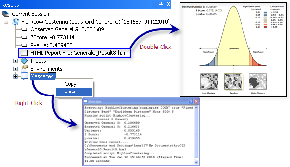
The High/Low Clustering tool returns four values: Observed General G, Expected General G, z-score, and p-value. These values are accessible from the Results window and are also passed as derived output values for potential use in models or scripts. Optionally, this tool will create an HTML file with a graphical summary of results. Double-clicking on the HTML file in the Results window will open the HTML file in the default Internet browser. Right-clicking on the Messages entry in the Results window and selecting View will display the results in a Message dialog box.

Frequently asked questions
Q: Results from the Hot Spot Analysis (Getis-Ord Gi*) tool indicate statistically significant hot spots. Why aren't results from the High/Low Clustering (Getis-Ord General G) tool statistically significant too?
A: Global statistics like the High/Low Clustering (Getis-Ord General G) tool assess the overall pattern and trend of your data. They are most effective when the spatial pattern is consistent across the study area. Local statistics tools (like Hot Spot Analysis) assess each feature within the context of neighboring features and compare the local situation to the global situation. Consider an example. When you compute a mean or average for a set of values, you are also computing a global statistic. If all the values are near 20, the mean will also be near 20, and that result will be a very good representation/summary of the dataset as a whole. But if half of the values are near 1 and the other half of the values are near 100, the mean will be near 50. There might not be any data values anywhere near 50, so the mean value is not a good representation/summary of the dataset as a whole. If you create a histogram of the data values, however, you will see the bimodal distribution. Similarly, global spatial statistics, including the High/Low Clustering tool, are most effective when the spatial processes being measured are consistent across the study area. Results will then be a good representation/summary of the overall spatial pattern. For more information, see Getis and Ord (1992), cited below, and the analysis of SIDS they present.
Q: Why are the results from the High/Low Clustering (Getis-Ord General G) tool different than the results from the Spatial Autocorrelation (Global Moran's I) tool?
A: See the table above. These tools measure different spatial patterns.
Q: Can you compare the z-scores or p-values from this tool to results from an analysis of a different study area?
A: Results really are not comparable unless the study area and parameters used for analysis are fixed (the same for all the analyses you want to compare). If the study area, however, comprises a fixed set of polygons, and the analysis parameters are fixed, you can compare z-scores for a particular attribute over time. Suppose, for example, you want to analyze trends in clustering of over-the-counter (OTC) medication purchases at the tract level for a particular county. You could run High/Low Clustering for each time period, then create a line graph of the results. If you found that the z-scores were statistically significant and increasing, you could conclude that the intensity of spatial clustering for high OTC purchases was increasing.
Q: Does feature size impact analysis?
A: The size of your features can affect your results. If your large polygons, for example, tend to have low values and your smaller polygons tend to have high values, even if the concentration of highs and lows are equally concentrated, the observed General G index may be higher than the expected General G index, because there are more pairs of small polygons within the specified distance.
Potential applications
- Look for unexpected spikes in the number of emergency room visits, which might indicate an outbreak of a local or regional health problem.
- Comparing the spatial pattern of different types of retail within a city to see which types cluster with competition to take advantage of comparison shopping (automobile dealerships, for example) and which types repel competition (fitness centers/gyms, for example).
- Summarizing the level at which spatial phenomena cluster to examine changes at different times or in different locations. For example, it is known that cities and their populations cluster. Using High/Low Clustering analysis, you can compare the level of population clustering within a single city over time (analysis of urban growth and density).
Additional resources
Getis, Arthur, and J. K. Ord. "The Analysis of Spatial Association by Use of Distance Statistics." Geographical Analysis 24, no. 3. 1992.
Mitchell, Andy. The ESRI Guide to GIS Analysis, Volume 2. ESRI Press, 2005.