The Multi-Distance Spatial Cluster Analysis tool, based on Ripley's K-function, is another way to analyze the spatial pattern of incident point data. A distinguishing feature of this method from others in this toolset (Spatial Autocorrelation and Hot Spot Analysis) is that it summarizes spatial dependence (feature clustering or feature dispersion) over a range of distances. In many feature pattern analysis studies, the selection of an appropriate scale of analysis is required. For example, a Distance Band or Threshold Distance is often needed for the analysis. When exploring spatial patterns at multiple distances and spatial scales, patterns change, often reflecting the dominance of particular spatial processes at work. Ripley's K-function illustrates how the spatial clustering or dispersion of feature centroids changes when the neighborhood size changes.
When using this tool, specify the number of distances to evaluate and, optionally, a starting distance and/or distance increment. With this information, the tool computes the average number of neighboring features associated with each feature; neighboring features are those closer than the distance being evaluated. As the evaluation distance increases, each feature will typically have more neighbors. If the average number of neighbors for a particular evaluation distance is higher/larger than the average concentration of features throughout the study area, the distribution is considered clustered at that distance.
Use this tool when you are interested in examining how the clustering/dispersion of your features changes at different distances (different scales of analysis).
Calculations
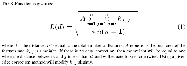
A number of variations of Ripley's original K-function have been suggested. Here, a common transformation of the K-function, often referred to as L(d), is implemented:

The default Beginning Distance and Distance Increment values are computed as follows:
- We always know the Number of Distance Bands (the default value is 10). We will use this Iterations value to compute a default Distance Increment if one isn't provided.
- We initially compute a Maximum Distance value as 25 percent of the maximum extent length of a minimum enclosing rectangle around the input features. If the Boundary Correction Method is REDUCE_ANALYSIS_AREA, then the Maximum Distance is set to the larger of either 25 percent of the maximum extent length or 50 percent of the minimum extent length of the minimum enclosing rectangle.
- If a Beginning Distance is provided, the Distance Increment is (Maximum Distance - Beginning Distance) / Iterations.
- If no Beginning Distance is provided, the Distance Increment is Max Distance / Iterations and the Beginning Distance is set to the Distance Increment value.
Interpreting unweighted K-function results
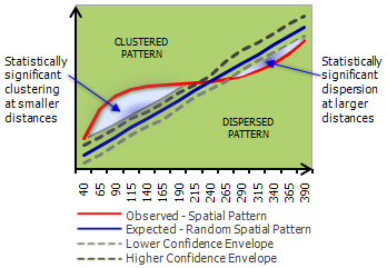
When the observed K value is larger than the expected K value for a particular distance, the distribution is more clustered than a random distribution at that distance (scale of analysis). When the observed K value is smaller than the expected K value, the distribution is more dispersed than a random distribution at that distance. When the observed K value is larger than the upper confidence envelope (HiConfEnv) value, spatial clustering for that distance is statistically significant. When the observed K value is smaller than the lower confidence envelope (LwConfEnv) value, spatial dispersion for that distance is statistically significant.
When no Weight Field is specified, the confidence envelope is constructed by distributing points randomly in the study area and calculating k for that distribution. Each random distribution of the points is called a "permutation". If 99 permutations is selected, for example, the tool will randomly distribute the set of points 99 times for each iteration. If 99_PERMUTATIONS is selected, for example, the tool will randomly distribute the set of points 99 times for each iteration. After distributing the points 99 times the tool selects, for each distance, the k value that deviated above and below the Expected k value by the greatest amount; these values become the confidence interval. The confidence envelopes tend to follow (have the same shape and location) as the blue Expected K line for unweighted K.

Interpreting weighted K-function results
The K-function always evaluates feature spatial distribution in relation to Complete Spatial Randomness (CSR), even when a Weight Field is provided. You can think of the weight as representing the number of coincident features at each feature location. For example, a feature with a weight of 3 may be interpreted as 3 coincident features. There is one difference, however: a feature cannot be its own neighbor. Consequently, you would get a different result for a dataset where there are 3 individual coincident points with a weight of 1 (all would be counted as neighbors of each other) than you would for a dataset with a single point with a weight of 3 (a feature is not counted as a neighbor of itself). Results from the weighted K-function will always be more clustered than results without a weight field. It is useful to run the K-function on the points without a weight to get a baseline indicating how much clustering is associated with feature locations alone. You can then compare the baseline to weighted results to get a feel for how much additional clustering or dispersion is added when the weight is considered. The weighted K-function shows the clustering (dispersion) over and above (under and below) that which it would obtain from the unweighted pattern. In fact, instead of CSR, you can use results from the unweighted K-function to represent the expected pattern (with its own confidence envelope). There are two possible null hypotheses in this case:
- The pattern of weighted features is not significantly more clustered (dispersed) than the underlying pattern of those features. You reject the null hypothesis if the observed weighted results fall outside the unweighted results confidence envelope.
- The pattern of weighted points is more clustered (dispersed) than chance would have it. You reject the null hypothesis if the observed unweighted results fall within the confidence envelope for the weighted K-function results.
When a Weight Field is specified, only the weight values are randomly redistributed to compute confidence envelopes; the point locations remain fixed. In essence, when a Weight Field is specified, locations remain fixed and the tool evaluates the clustering of feature values in space. Because results are strongly structured by the fixed locations of the features, for weighted K analyses the confidence envelope tends to follow/mirror the red Observed K line.
Additional resources
Bailey, T. C., and A. C. Gatrell. Interactive Spatial Data Analysis. Longman Scientific & Technical, Harlow, U.K. 395 pp. 1995.
Boots, B., and A. Getis. Point Pattern Analysis. Sage University Paper Series on Quantitative Applications in the Social Sciences, series no. 07–001. Sage Publications. 1988.
Getis, A. Interactive Modeling Using Second-Order Analysis. Environment and Planning A, 16: 173–183. 1984.
Mitchell, Andy. The ESRI Guide to GIS Analysis, Volume 2. ESRI Press, 2005.