Regression analysis is used to understand, model, predict, and/or explain complex phenomena. It helps you answer why questions like "Why are there places in the United States with test scores that are consistently above the national average?" or "Why are there areas of the city with such high rates of residential burglary?" You might use regression analysis to explain childhood obesity, for example, using a set of related variables such as income, education, and accessibility to healthy food.
Typically, regression analysis helps you answer these why questions so that you can do something about them. If, for example, you discover that childhood obesity is lower in schools that serve fresh fruits and vegetables at lunch, you can use that information to guide policy and make decisions about school lunch programs. Likewise, knowing the variables that help explain high crime rates can allow you to make predictions about future crime so that prevention resources can be allocated more effectively.
These are the things they do tell you about regression analysis.
What they don't tell you about regression analysis is that it isn't always easy to find a set of explanatory variables that will allow you to answer your question or to explain the complex phenomenon you are trying to model. Childhood obesity, crime, test scores, and almost all the things that you might want to model using regression analysis are complicated issues that rarely have simple answers. Chances are, if you have ever tried to build your own regression model, this is nothing new to you.
Fortunately, when you run the Ordinary Least Squares (OLS) regression tool, you are presented with a set of diagnostics that can help you figure out whether you have a properly specified model; a properly specified model is one you can trust. This document examines the six checks you'll want to pass to have confidence in your model. Those six checks, and the techniques that you can use to solve some of the most common regression analysis problems, are resources that can definitely make your work easier.
Getting started
Choosing the variable you want to understand, predict, or model is your first task. This variable is known as the dependent variable. Childhood obesity, crime, and test scores would be the dependent variables being modeled in the examples described above.
Next you have to decide which factors might help explain your dependent variable. These variables are known as the explanatory variables. In the childhood obesity example, the explanatory variables might be things such as income, education, and accessibility to healthy food. You will need to do your research here to identify all the explanatory variables that might be important; consult theory and existing literature, talk to experts, and always rely on your common sense. The preliminary research you do up front will greatly increase your chances of finding a good model.
With the dependent variable and the candidate explanatory variables selected, you are ready to run your analysis. Always start your regression analysis with Ordinary Least Squares or Exploratory Regression because these tools perform important diagnostic tests that let you know if you've found a useful model or if you still have some work to do.
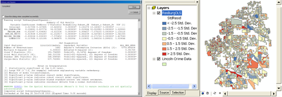
The OLS tool generates several outputs including a map of the regression residuals and a summary report. The regression residuals map shows the under- and overpredictions from your model, and analyzing this map is an important step in finding a good model. The summary report is largely numeric and includes all the diagnostics you will use when going through the six checks below.
The six checks
Check 1: Are these explanatory variables helping my model?
After consulting theory and existing research, you will have identified a set of candidate explanatory variables. You'll have good reasons for including each one in your model. However, after running your model, you'll find that some of your explanatory variables are statistically significant and some are not.
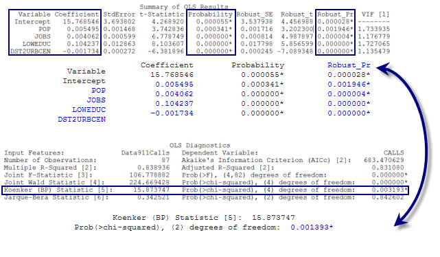
How will you know which explanatory variables are significant? The OLS tool calculates a coefficient for each explanatory variable in the model and performs a statistical test to determine whether that variable is helping your model or not. The statistical test computes the probability that the coefficient is actually zero. If the coefficient is zero (or very near zero), the associated explanatory variable is not helping your model. When the statistical test returns a small probability (p-value) for a particular explanatory variable, on the other hand, it indicates that it is unlikely (there is a small probability) that the coefficient is zero. When the probability is smaller than 0.05, an asterisk next to the probability on the OLS summary report indicates the associated explanatory variable is important to your model (in other words, its coefficient is statistically significant at the 95 percent confidence level). So you are looking for explanatory variables associated with statistically significant probabilities (look for ones with asterisks).
The OLS tool computes both the probability and the robust probability for each explanatory variable. With spatial data, it is not unusual for the relationships you are modeling to vary across the study area. These relationships are characterized as nonstationary. When the relationships are nonstationary, you can only trust robust probabilities to tell you whether an explanatory variable is statistically significant.
How will you know if the relationships in your model are nonstationary? Another statistical test included in the OLS summary report is the Koenker (Koenker's studentized Breusch-Pagan) statistic for nonstationarity. An asterisk next to the Koenker p-value indicates the relationships you are modeling exhibit statistically significant nonstationarity, so be sure to consult the robust probabilities.
Typically you will remove explanatory variables from your model if they are not statistically significant. However, if theory indicates a variable is very important, or if a particular variable is the focus of your analysis, you might retain it even if it's not statistically significant.
Check 2: Are the relationships what I expected?
Not only is it important to determine whether an explanatory variable is actually helping your model, but you also want to check the sign (+/-) associated with each coefficient to make sure the relationship is what you were expecting. The sign of the explanatory variable coefficient indicates whether the relationship is positive or negative. Suppose you were modeling crime, for example, and one of your explanatory variables is average neighborhood income. If the coefficient for the income variable is a negative number, it means that crimes tend to decrease as neighborhood incomes increase (a negative relationship). If you were modeling childhood obesity and the accessibility to fast food variable had a positive coefficient, it would indicate that childhood obesity tends to increase as access to fast food increases (a positive relationship).
When you create your list of candidate explanatory variables, you should include for each variable the relationship (positive or negative) you are expecting. You would have a hard time trusting a model reporting relationships that don't match with theory and/or common sense. Suppose you were building a model to predict forest fire frequencies and your regression model returned a positive coefficient for the precipitation variable. You probably wouldn't expect forest fires to increase in locations with lots of rain.
Unexpected coefficient signs often indicate other problems with your model that will surface as you continue working through the six checks. You can only trust the sign and strength of your explanatory variable coefficients if your model passes all of these. If you do find a model that passes all the checks despite the unexpected coefficient sign, you may have discovered an opportunity to learn something new. Perhaps there is a positive relationship between forest fire frequency and precipitation because the primary source of forest fires in your study area is lightning. It may be worthwhile to try to obtain data about lightning for your study area to see if it improves model performance.
Check 3: Are any of the explanatory variables redundant?
When choosing explanatory variables to include in your analysis, look for variables that get at different aspects of what you are trying to model; avoid variables that are telling the same story. For example, if you were trying to model home values, you probably wouldn't include explanatory variables for both home square footage and number of bedrooms. Both of these variables relate to the size of the home, and including both could make your model unstable. Ultimately, you cannot trust a model that includes redundant variables.
How will you know if two or more variables are redundant? Fortunately, whenever you have more than two explanatory variables, the OLS tool computes a Variance Inflation Factor (VIF) for each variable. The VIF value is a measure of variable redundancy and can help you decide which variables can be removed from your model without jeopardizing explanatory power. As a rule of thumb, a VIF value above 7.5 is problematic. If you have two or more variables with VIF values above 7.5, you should remove them one at a time and rerun OLS until the redundancy is gone. Keep in mind that you do not want to remove all the variables with high VIF values. In the example of modeling home values, square footage and number of bedrooms would likely both have inflated VIF values. As soon as you remove one of those two variables, however, the redundancy is eliminated. Including a variable that reflects home size is important; you just don't want to model that aspect of home values redundantly.
Check 4: Is my model biased?
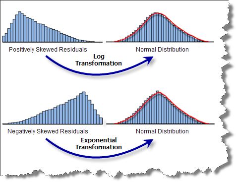
This may seem like a tricky question, but the answer is actually very simple. When you have a properly specified OLS model, the model residuals (the over- and underpredictions) are normally distributed with a mean of zero (think bell curve). When your model is biased, however, the distribution of the residuals is unbalanced as shown below. You cannot fully trust predicted results when the model is biased. Luckily, there are several strategies to help you correct this problem.
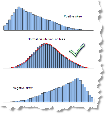
A statistically significant Jarque-Bera diagnostic (look for the asterisk) indicates your model is biased. Sometimes your model is doing a good job for low values but is not predicting well for high values (or vice versa). With the childhood obesity example, this would mean that, in locations with low childhood obesity, the model is doing a great job, but in areas with high childhood obesity, the predictions are off. Model bias can also be the result of outliers that are influencing model estimation.
To help you resolve model bias, create a scatterplot matrix for all your model variables. A nonlinear relationship between your dependent variable and one of your explanatory variables is a common cause of model bias. These might look like a curved line in the scatterplot matrix. Linear relationships look like diagonal lines.
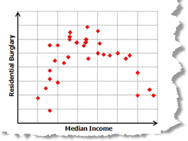
If you see that your dependent variable has a nonlinear relationship with one of your explanatory variables, you have some work to do. OLS is a linear regression method that assumes the relationships you are modeling are linear. When they aren't, you can try transforming your variables to see if this creates relationships that are more linear. Common transformations include log and exponential. Check the Show Histograms option (which turns it on) in the Create Scatterplot Matrix wizard to include a histogram for each variable in the scatterplot matrix. If some of your explanatory variables are strongly skewed, you might be able to remove model bias by transforming them as well.
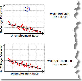
The scatterplot matrix will also reveal data outliers. To see whether an outlier is impacting your model, try running OLS both with and without an outlier and check to see how much it changes model performance and whether removing it corrects model bias. In some instances (especially if you think that the outliers represent bad data), you might be able to drop the outliers from your analysis.
Check 5: Have I found all the key explanatory variables?
Often you go into an analysis with hypotheses about which variables are going to be important predictors. Maybe you believe 5 particular variables will produce a good model, or maybe you have a firm list of 10 variables you think might be related. While it is important to approach regression analysis with a hypothesis, it is also important to allow your creativity and insight to help you dig deeper. Resist the inclination to limit yourself to your initial variable list, and try to consider all the possible variables that might impact what you are modeling. Create thematic maps of each of your candidate explanatory variables and compare those to a map of your dependent variable. Hit the books again and scan the relevant literature. Use your intuition to look for relationships in your mapped data. Definitely try to come up with as many candidate spatial variables as you can, such as distance from the urban center, proximity to major highways, or access to large bodies of water. These kinds of variables will be especially important for analyses where you believe geographic processes influence relationships in your data. Until you find explanatory variables that effectively capture the spatial structure in your dependent variable, in fact, your model will be missing key explanatory variables and you will not be able to pass all the diagnostic checks outlined here.
Evidence that you are missing one or more key explanatory variables is statistically significant spatial autocorrelation of your model residuals. In regression analysis, issues with spatially autocorrelated residuals usually takes the form of clustering: the overpredictions cluster together and the underpredictions cluster together. How will you know if you have statistically significant spatial autocorrelation in your model residuals? Running the Spatial Autocorrelation tool on your regression residuals will tell you if you have a problem with spatial autocorrelation. A statistically significant z-score indicates you are missing key explanatory variables from your model.
Finding those missing explanatory variables is often as much an art as a science. Try these strategies to see if they provide any clues:
Examine the OLS residual map
The standard output from OLS is a map of the model residuals. Red areas indicate the actual values (your dependent variable) are larger than your model predicted they would be. Blue areas show where the actual values are lower than predicted. Sometimes just seeing the residual map will give you a clue about what might be missing. If you notice that you are consistently overpredicting in urbanized areas, for example, you might want to consider adding a variable that reflects distance to urban centers. If it looks like overpredictions are associated with mountain peaks or valley bottoms, perhaps you need an elevation variable. Do you see regional clusters, or can you recognize trends in your data? If so, creating a dummy variable to capture these regional differences may be effective. The classic example for a dummy variable is one that distinguishes urban and rural features. By assigning all rural features a value of 1 and all other features a value of 0, you may be able to capture spatial relationships in the landscape that could be important to your model. Sometimes creating a hot spot map of model residuals will help you visualize broad regional patterns.
Figuring out the missing spatial variables not only has the potential to improve your model, but this process can also help you better understand the phenomenon you are modeling in new and innovative ways.
Examine nonstationarity
You can also try running Geographically Weighted Regression and creating coefficient surfaces for each of your explanatory variables and/or maps of the local R2 values. Select the OLS model that is performing well (one with a high adjusted R2 value that is passing all or most all the other diagnostic checks). Because GWR creates a regression equation for each feature in your study area, the coefficient surfaces illustrate how the relationships between the dependent variable and each explanatory variable fluctuate geographically; the map of local R2 values shows variations in model explanatory power. Sometimes seeing these geographic variations will spark ideas about what variables might be missing: a dip in explanatory power near major freeways, a decline with distance from the coast, a change in the sign of the coefficients near an industrial region, or a strong east to west trend or boundary—all these would be clues about spatial variables that may improve your model.
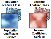
When you examine the coefficient surfaces, be on the lookout for explanatory variables with coefficients that change sign from positive to negative. This is important because OLS will likely discount the predictive potential of these highly nonstationary variables. Consider, for example, the relationship between childhood obesity and access to healthy food options. It may be that in low-income areas with poorer access to cars, being far away from a supermarket is a real barrier to making healthy food choices. In high-income areas with better access to vehicles, however, having a supermarket within walking distance might actually be undesirable; the distance to the supermarket might not act as a barrier to buying healthy foods at all. While GWR is capable of modeling these types of complex relationships, OLS is not. OLS is a global model and is expecting variable relationships to be consistent (stationary) across the study area. When coefficients change sign, they cancel each other out. Think of it as (+1) + (-1) = 0. When you find variables where the coefficients are changing dramatically, especially if they are changing signs, you should keep them in your model even if they are not statistically significant. These types of variables will be effective when you move to GWR.
Try fitting OLS to smaller subset study areas
GWR is tremendously useful when dealing with nonstationarity, and it can be tempting to move directly to GWR without first finding a properly specified OLS model. Unfortunately, GWR doesn't have all the great diagnostics to help you figure out whether your explanatory variables are statistically significant, your residuals are normally distributed, or, ultimately, you have a good model. GWR will not fix an improperly specified model unless you can be sure that the only reason your OLS model is failing the six checks is the direct result of nonstationarity. Evidence of nonstationarity would be finding explanatory variables that have a strong positive relationship in some parts of the study area and a strong negative relationship in other parts. Sometimes the issue isn't with individual explanatory variables but with the set of explanatory variables used in the model. It may be that one set of variables provides a great model for one part of the study area, but another set of different variables works best everywhere else. To see if this is the case, you can select several smaller subset study areas and try to fit OLS models to each of these. Select your subset areas based on the processes you think may be related to your model (high- versus low-income areas, old versus new housing). Alternatively, select areas based on the GWR map of local R2 values; the locations with poor model performance might be modeled better using a different set of explanatory variables.
If you do find properly specified OLS models in several small study areas, you can conclude that nonstationarity is the culprit and move to GWR using the full set of explanatory variables you found from all subset area models. If you don't find properly specified models in the smaller subset areas, it may be that you are trying to model something that is too complex to be reduced to a simple series of numeric measurements and linear relationships. In that case, you probably need to explore alternative analytic methods.
All of this can be a bit of work, but it is also a great exercise in exploratory data analysis and will help you understand your data better, find new variables to use, and may even result in a great model.
Check 6: How well am I explaining my dependent variable?
Now it's finally time to evaluate model performance. The adjusted R2 value is an important measure of how well your explanatory variables are modeling your dependent variable. The R2 value is also one of the first things they tell you about regression analysis. So why are we leaving this important check until the end? What they don't tell you is that you cannot trust your R2 value unless you have passed all the other checks listed above. If your model is biased, it may be performing well in some areas or with a particular range of your dependent variable values, but otherwise not performing well at all. The R2 value doesn't reflect that. Likewise, if you have spatial autocorrelation of your residuals, you cannot trust the coefficient relationships from your model. With redundant explanatory variables you can get extremely high R2 values, but your model will be unstable; it will not reflect the true relationships you are trying to model and might produce completely different results with the addition of even a single observation.
Once you have gone through the other checks and feel confident that you have met all the necessary criteria, however, it is time to figure out how well your model is explaining the values for your dependent variable by assessing the adjusted R2 value. R2 values range between 0 and 1 and represent a percentage. Suppose you are modeling crime rates and find a model that passes all five of the previous checks with an adjusted R2 value of 0.65. This lets you know that the explanatory variables in your model are telling 65 percent of the crime rate story (more technically, the model is explaining 65 percent of the variation in the crime rate dependent variable). Adjusted R2 values have to be judged rather subjectively. In some areas of science, explaining 23 percent of a complex phenomenon will be very exciting. In other fields, an R2 value may need to be closer to 80 or 90 percent before it gets anyone's attention. Either way, the adjusted R2 value will help you judge how well your model is performing.
Another important diagnostic to help you assess model performance is the corrected Akaike's information criterion (AICc). The AICc value is a useful measure for comparing multiple models. For example, you might want to try modeling student test scores using several different sets of explanatory variables. In one model you might use only demographic variables, while in another model you might select variables relating to the school and classroom, such as per-student spending and teacher-to-student ratios. As long as the dependent variable for all the models being compared is the same (in this case, student test scores), you can use the AICc values from each model to determine which performs better. The model with the smaller AICc value provides a better fit to the observed data.
And don't forget . . .
Keep in mind as you are going through these steps of building a properly specified regression model that the goal of your analysis is ultimately to understand your data and use that understanding to solve problems and answer questions. The truth is that you could try a number of models (with and without transformed variables), explore several small study areas, analyze your coefficient surfaces ...and still not find a properly specified OLS model. But—and this is important—you will still be contributing to the body of knowledge on the phenomenon you are modeling. If the model you hypothesized would be a great predictor turns out not to be significant at all, discovering that is incredibly helpful information. If one of the variables you thought would be strong has a positive relationship in some areas and a negative relationship in others, knowing about this certainly increases your understanding of the issue. The work that you do here, trying to find a good model using OLS and then applying GWR to explore regional variation among the variables in your model, is always going to be valuable.
For more information about regression analysis, check out the Spatial Statistics Resources page.