Interpreting GWR results

Output generated from the Geographically Weighted Regression (GWR) tool includes the following:

1. Output feature class
2. Optional coefficient raster surfaces
3. Message window report of overall model results
4. Supplementary table showing model variables and diagnostic results
5. Prediction output feature class

Each of the above outputs is shown and described below as a series of steps for running GWR and interpreting GWR results. You will typically begin your regression analysis with Ordinary Least Squares (OLS). See Regression Analysis Basics and Interpreting OLS Regression Results for more information. A common approach to regression analysis is to identify the very best OLS model possible before moving to GWR. This approach provides the context for the steps below.

(A) Open the Results window, if necessary. After you have identified one or more candidate regression models using the OLS regression tool, run those models using GWR. Exclude from your GWR model any regional binary (dummy) variables, as these will create problems with local multicollinearity and are not needed with GWR. You will need to provide an Input feature class with the Dependent variable you want to model/explain/predict and all the model Explanatory variables. You will also need to provide a path name for the Output feature class, a Kernel type (either fixed or adaptive), and a Bandwidth method (AICc, CV, or user-provided value). If, for Bandwidth method, you select BANDWIDTH_PARAMETER, you will need to provided a specific Distance (for a fixed Kernel Type) or a specific Number of neighbors (for an adaptive Kernel Type). You can also provide values for the optional parameters described in the GWR tool documentation. One especially interesting optional parameter is the Coefficient raster workspace. When you provide a folder path name for this parameter, the GWR tool will create coefficient raster surfaces (described below) for the model intercept and each explanatory variable.

GWR Tool Dialog Box

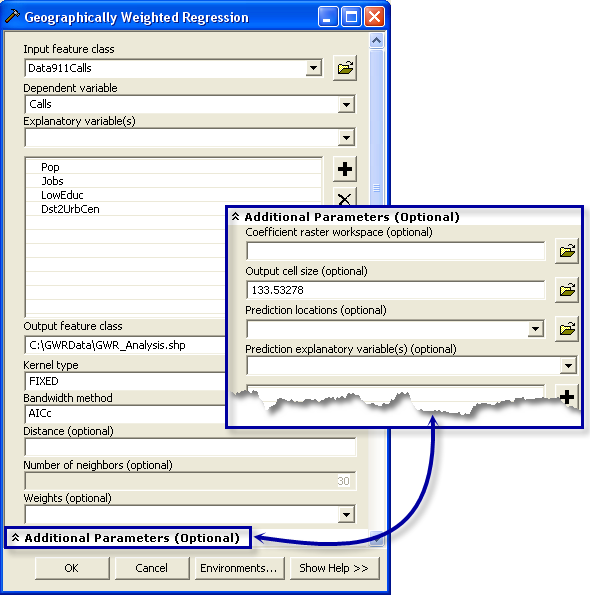
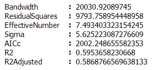
(B) Examine the statistical summary report written to the Results window. Right-clicking the Messages entry in the Results window and selecting View will display the GWR summary report in a Message dialog box. If you execute this tool in the foreground, the summary report will also be displayed in the progress dialog box. Each of the diagnostics reported is described below.

1. Bandwidth or Neighbors: This is the bandwidth or number of neighbors used for each local estimation and is perhaps the most important parameter for Geographically Weighted Regression. It controls the degree of smoothing in the model. Typically, you will let the program choose a bandwidth or neighbor value for you by selecting the corrected Akaike Information Criterion (AICc) or Cross Validation (CV) for the Bandwidth method parameter. Both of these options try to identify an optimal fixed distance or optimal adaptive number of neighbors. Since the criteria for what is considered to be optimal are different for AICc than for CV, it is common to get a different optimal value. You may also provide an exact fixed distance or a particular number of neighbors by selecting As specified below for the Bandwidth methodYou may also provide an exact fixed distance or a particular number of neighbors by selecting BANDWIDTH_PARAMETER for the Bandwidth method

   The bandwidth units depend on the specified Kernel type. If you select FIXED, the bandwidth value will reflect a distance in the same units as the Input feature class (for example, if the input feature class is projected using UTM coordinates, the distance reported will be in meters). If you select ADAPTIVE, the bandwidth distance will change according to the spatial density of features in the Input feature class. The bandwidth becomes a function of the number of nearest neighbors such that each local estimation is based on the same number of features. Instead of a specific distance, the number of neighbors used for the analysis is reported.

2. ResidualSquares: This is the sum of the squared residuals in the model (the residual being the difference between an observed y value and its estimated value returned by the GWR model). The smaller this measure, the closer the fit of the GWR model to the observed data. This value is used in a number of other diagnostic measures.
3. EffectiveNumber: This value reflects a tradeoff between the variance of the fitted values and the bias in the coefficient estimates and is related to the choice of bandwidth. As the bandwidth approaches infinity, the geographic weights for every observation approach 1, and the coefficient estimates will be very close to those for a global OLS model. For very large bandwidths, the effective number of coefficients approaches the actual number; local coefficient estimates will have a small variance but will be quite biased. Conversely, as the bandwidth approaches zero, the geographic weights for every observation approach zero with the exception of the regression point itself. For extremely small bandwidths, the effective number of coefficients is the number of observations, and the local coefficient estimates will have a large variance but a low bias. The effective number is used to compute a number of diagnostic measures.
4. Sigma: This value is the square root of the normalized residual sum of squares, where the residual sum of squares is divided by the effective degrees of freedom of the residual. This is the estimated standard deviation for the residuals. Smaller values of this statistic are preferable. Sigma is used for AICc computations.
5. AICc: This is a measure of model performance and is helpful for comparing different regression models. Taking into account model complexity, the model with the lower AICc value provides a better fit to the observed data. AICc is not an absolute measure of goodness of fit but is useful for comparing models with different explanatory variables as long as they apply to the same dependent variable. If the AICc values for two models differ by more than 3, the model with the lower AICc is held to be better. Comparing the GWR AICc value to the OLS AICc value is one way to assess the benefits of moving from a global model (OLS) to a local regression model (GWR).
6. R2: R-Squared is a measure of goodness of fit. Its value varies from 0.0 to 1.0, with higher values being preferable. It may be interpreted as the proportion of dependent variable variance accounted for by the regression model. The denominator for the R2 computation is the sum of squared dependent variable values. Adding an extra explanatory variable to the model does not alter the denominator but does alter the numerator; this gives the impression of improvement in model fit that may not be real. See Adjusted R2 below.
7. R2Adjusted: Because of the problem described above for the R2 value, calculations for the adjusted R-squared value normalize the numerator and denominator by their degrees of freedom. This has the effect of compensating for the number of variables in a model, and consequently, the Adjusted R2 value is almost always smaller than the R2 value. However, in making this adjustment, you lose the interpretation of the value as a proportion of the variance explained. In GWR, the effective number of degrees of freedom is a function of the bandwidth, so the adjustment may be quite marked in comparison to a global model like OLS. For this reason, the AICc is preferred as a means of comparing models.

GWR tool execution output

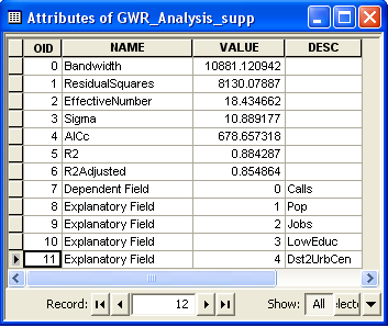
Message window diagnostics are written to a supplementary table (_supp) along with summary information about model variables and parameters.

GWR _supp output table

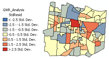
(C) Examine the output feature class residuals.

Over- and underpredictions for a well-specified regression model will be randomly distributed. Clustering of over- and/or underpredictions is evidence that you are missing at least one key explanatory variable. Examine the patterns in your OLS and GWR model residuals to see if they provide clues about what those missing variables might be. Run the Spatial Autocorrelation (Moran's I) tool on the regression residuals to ensure that they are spatially random. Statistically significant clustering of high and/or low residuals (model under- and overpredictions) indicates that the GWR model is misspecified.

GWR feature class output with rendered residuals

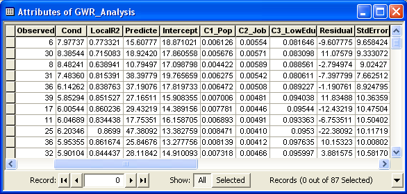
In addition to regression residuals, the Output feature class includes fields for observed and predicted y values, condition number (cond), Local R2, explanatory variable coefficients, and standard errors:

1. Condition Number: This diagnostic evaluates local multicollinearity. In the presence of strong local multicollinearity, results become unstable. Results associated with condition numbers larger than 30 may be unreliable.
2. Local R2: These values range between 0.0 and 1.0 and indicate how well the local regression model fits observed y values. Very low values indicate that the local model is performing poorly. Mapping the Local R2 values to see where GWR predicts well and where it predicts poorly may provide clues about important variables that may be missing from the regression model.
3. Predicted: These are the estimated (or fitted) y values computed by GWR.
4. Residuals: To obtain the residual values, the fitted y values are subtracted from the observed y values. Standardized residuals have a mean of zero and a standard deviation of 1. A cold-to-hot rendered map of standardized residuals is automatically added to the table of contents when GWR is executed in ArcMap.
5. Coefficient Standard Error: These values measure the reliability of each coefficient estimate. Confidence in those estimates is higher when standard errors are small in relation to the actual coefficient values. Large standard errors may indicate problems with local multicollinearity.

Output feature class results

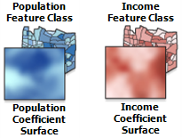
(D) Examine the coefficient raster surfaces created by GWR (and/or with polygon data, a graduated color rendering of the feature-level coefficients) to better understand regional variation in the model explanatory variables. When you use GWR to model some variable (the dependent variable) you are generally interested in predicting values or understanding the factors that contribute to dependent variable outcomes. You are also interested, however, in examining how spatially consistent (stationary) relationships between the dependent variable and each explanatory variable are across the study area. Examining the coefficient distribution as a surface shows where and how much variation is present. You can use your understanding of this variation to inform policy:

• Statistically significant global variables that exhibit little regional variation inform regionwide policy.
• Statistically significant global variables that exhibit strong regional variation inform local policy.
• Some variables may not be globally significant, because in some regions, they are positively related, and in others are negatively related.

Spatial heterogeneity is revealed in output coefficient raster surfaces.

(E) Map GWR predictions. GWR can be used for prediction when it is applied to sampled data. Specify a feature class containing all the explanatory variables for locations where the dependent variable is unknown. GWR calibrates the regression equation using known dependent variable values from the Input feature class, then creates a new Output feature class with dependent variable estimates.