Available with Standard or Advanced license.
The parcel fabric adjustment is a least-squares adjustment that is run on a selection of parcels to incrementally improve the positional accuracy of the parcel corner points. While COGO dimensions accurately define the shape of a parcel, a parcel fabric adjustment with survey control points accurately defines the spatial location of a parcel.
Understanding a least-squares adjustment
A single observation (bearing and distance) from an existing point can be used to compute the coordinates for a new point. However, relying on a single observation is risky, since there is no way to tell whether the measurement is correct. A second measurement from the same or another existing point will confirm, or check, the coordinates defined by the first measurement. Generally, the more measurements fixing the coordinates of a point, the more reliable the coordinates. These additional measurements are called redundant measurements.
All measurements contain some degree of error. Therefore, each measurement will compute slightly different coordinates for the same survey point. For practical reasons, there should be one coordinate location for a survey point. A single, best estimate coordinate can be derived by computing a weighted average of the additional or redundant measurements, with each weight defined by the measurement accuracy.
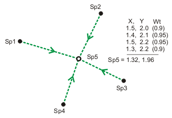
Although the weighted average approach works for a single point, it is not sufficient to compute the coordinates for multiple points in a network such as the parcel fabric. A more advanced method is needed to account for the numerous possible measurement paths between the points. The techniques and algorithms in a least-squares adjustment provide the most rigorous and widely accepted solution for processing a network of measurements and points.
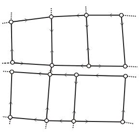
A least-squares adjustment is a mathematical procedure based on the theory of probability that derives the statistically most likely coordinate location of points defined by multiple measurements in a network. In mathematical terms, a least-squares adjustment defines a best-fit solution for weighted measurements by finding a minimum for the sum of the squares of the measurement residuals. A measurement residual is the amount needed to correct a measurement for it to fit into the best-fit solution found by the least-squares adjustment.
About the parcel fabric least-squares adjustment
A parcel fabric least-squares adjustment is run on a parcel fabric to incrementally improve the positional accuracy of parcel corner points. While COGO dimensions accurately define the shape of a parcel, and a least-squares adjustment with survey control points accurately defines the spatial location of a parcel.
The least-squares adjustment engine in the parcel fabric uses dimensions on parcel lines together with control points to estimate the statistically most likely coordinate location for every parcel point in the network. This description of the least-squares adjustment can be more easily understood by considering one traverse path between two control points in the fabric network. Fabric points P1 and P5 should be coincident with their corresponding control points CP1 and CP2. The least-squares adjustment adjusts the misclose error between P1 and CP1 as well as P5 and CP2 through the remaining points P2, P3, and P4 such that P1 and P5 become coincident with their control points. The coordinates of P2, P3, and P4 are adjusted into the best-fit solution and the lines are recalculated from the adjusted points. In the parcel fabric, accuracy on parcel lines acts as a weighting system in the least-squares adjustment. Lines with higher weights will adjust less than lines with lower weights. The higher the accuracy, the higher the weight on a parcel line. In the graphic below, the line between P2 and P3 has a high accuracy and thus a high weight. In the least-squares adjustment, line P2–P3 received proportionally less of an adjustment than the other lines in the traverse path.
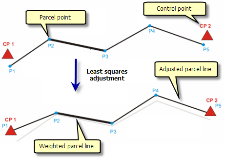
The residual differences between the original lines and the lines computed from the adjusted coordinates reveal how well the parcel lines fit among themselves and with the control points. A large residual suggests a problem with the parcel line itself or nearby parcel lines, since the original value required a significant change to fit into the best-fit solution.
The adjustment process
In the first step of the adjustment, transformation parameters between the coordinates of the control points and the corresponding coordinates of their underlying parcel points are determined. If the transformation residuals are within acceptable limits (the differences between the two coordinate systems), the transformation parameters are applied to all parcel fabric coordinates to transform them into the coordinates of the control system. Running a check fit on the control points displays these transformations residuals.
After the transformation, the bearing and distance of every parcel line is compared with the same bearing and distance of the line shapes computed in the transformed coordinate system (the coordinate system of the control points). This is done by calculating the difference between the bearing and distance computed from the transformed coordinates and the original bearing and distance. Any parcel line with a bearing and distance difference that exceeds the tolerances you specify in the Adjust Coordinates dialog box is reported in the adjustment report. After the coordinates of the parcel fabric have been transformed into the coordinates of the control system, the adjustment engine averages (computes a mean) the coordinates and determines the most optimal, best fit solution for all points in the network. The adjustment is a weighted least-squares adjustment, where parcels with a higher accuracy level (higher weight) adjust less than those parcels with lower accuracy level (lower weight).
Redundancy
A least-squares adjustment produces the most reliable results when there are redundant measurements in a network. Redundancy implies that there are repeated observations for a single measurement. Repeated observations validate the measurement network. A parcel fabric is a redundant measurement network.
In the graphic below, a single parcel has four lines and four points. Corner point 2 is defined by two lines (measurements).
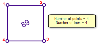
In the parcel fabric, corner point 2 from the same parcel is now defined by eight lines (measurements).
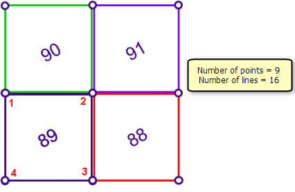
With the redundant eight lines defining the same point 2, it's now easier to identify a line that defines a coordinate for point 2 that is significantly different from the coordinates defined by the other lines. Thus, the more lines defining the same point coordinate, the more reliable the detection of outliers or inconsistent lines. The least-squares adjustment uses redundancy to identify those lines that do not fit with the best fit solution. Redundancy in the parcel fabric is created through common points and connectivity.
Handling basis of bearing
In the parcel fabric, bearings for the lines in each parcel are assumed to be on an azimuth for that parcel. Furthermore, each parcel may have to be separately rotated and scaled to fit with the datum and projection used in the parcel fabric. If internal angles are used for the traverse entry of a parcel, the angles are stored and bearings are computed for the lines based on an assumed azimuth. Bearings are required because the adjustment uses bearing equations, not angle equations, for the parcel lines.
When a parcel is joined to the fabric, the original dimensions are used to first calculate coordinates for the parcel corners on a local coordinate system. The first point in the parcel is given coordinates of 0.0 east and 0.0 north and the dimensions are used to compute all subsequent points. A Bowditch adjustment is used to distribute the misclose before computing the local coordinates.
During the joining process, unjoined parcel corner points are matched with their corresponding points in the fabric. Transformation parameters are calculated between the coordinates of the parcel and the coordinate system of the fabric. A Helmert transformation (rotation, scale, shift in x, and shift in y) is used. If more than two points are used in the joining, a least-squares procedure is used to determine the parameters. As points are joined, they are transformed into the network of the fabric and the differences or transformation residuals are displayed as dx (change in x) and dy (change in y) on the join dialog box. These residuals are a good indication of how well the parcels being joined are fitting into the surrounding parcel fabric.
After a parcel is joined, the rotation and scale factor (from the transformation) is stored with the parcel and is used by the least-squares adjustment in setting up the bearing equations. In the least-squares adjustment, parcel bearings are treated like a geodetic "direction set." The assumption is that the angles between each parcel line are correct, but the whole group of lines could be rotated slightly (basis of bearing). So the least-squares adjustment solves for corrections for x,y for every point and for a rotation correction or "orientation element" for each parcel.
The adjustment reports a rotation, scale factor, dx (change in x), and dy (change in y) for each parcel adjusted. Within a subdivision plan, the rotation and scale factor should be very similar for each parcel, and the dx and dy give an indication of change of shape for the parcel. If the adjustment is rerun, the rotation and scale for each parcel will be recalculated.