Available with Geostatistical Analyst license.
Disjunctive kriging requires that the data follow a bivariate normal distribution. Also, to develop probability and quantile maps, it's assumed that the data comes from a full multivariate normal distribution. To check for a univariate normal distribution, you can use normal QQ plots or histograms (neither of these checks guarantees that the data comes from a full multivariate normal distribution, but it is often reasonable to assume so if univariate normal distributions are detected using these diagnostic tools).
Consider the following probability statement:
f(p,h) = Prob[Z(s) ≤ zp, Z(s + h) ≤ zp],where zp is the standard normal quantile for some probability p.
For example, a familiar standard normal quantile occurs when p = 0.975, then zp = 1.96, and when p = 0.5, then zp = 0, and when p = 0.025, then zp = -1.96. The probability statement above takes a variable Z at location s and another variable Z at some other location s + h and gives the probability that they are both less than zp. This probability statement is a function f(p,h) depending on p (and consequently zp) and h. The function will also depend on the amount of autocorrelation between Z(s) and Z(s + h).
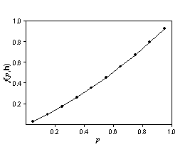
Assume that Z(s) and Z(s + h) have a bivariate normal distribution. If the autocorrelation is known, there are formulas for f(p,h). Suppose h is constant and only p changes. You would expect the function to look like this:


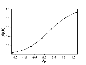
The second figure looks like a cumulative probability distribution. Now, suppose that p is fixed, and f(p,h) changes with h.
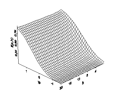
First, suppose that h is very small. In that case, Prob[Z(s) ≤ zp, Z(s + h) ≤ zp] is very nearly the same as Prob[Z(s) ≤ zp] = p. Next, suppose that h is very large. In that case, Prob[Z(s) ≤ zp, Z(s + h) ≤ zp] is very nearly the same as Prob[Z(s) ≤ zp] Prob[Z(s + h) ≤ zp] = p2 (because Z(s) and Z(s + h) are very nearly independent). Thus, for fixed p, you expect f(p,h) to vary between p and p2. Now, considering f(p,h) as a function of both p and the length of h, you might observe something similar to the following figure:

This function can be converted to semivariograms and covariance functions for indicators. If you note that Prob[Z(s) ≤ zp, Z(s + h) ≤ zp] = E[I(Z(s) ≤ zp)xI(Z(s + h) ≤ zp)], where I(statement) is the indicator function—is 1 if statement is true, otherwise it is 0—the covariance function for the indicators for fixed p is
CI(h;p) = f(p,h) –p2,and the semivariogram for indicators for fixed p is
γI(h;p) = p - f(p,h).Therefore, you can estimate the semivariogram and covariance function on the indicators of the original data and use these to obtain the expected semivariograms and covariance functions of indicators for various values of p.