Generalizing data involves many repetitive, labor-intensive tasks, so it is an ideal candidate for automation. However, the contextual and subjective nature of generalization makes it difficult to automate. The human brain is very adept at prioritizing and making contextual concessions simultaneously. It is much more difficult to instruct a computer to do this with a series of discrete commands.
The geoprocessing environment in ArcGIS is well suited to establishing a generalization framework, since it can manage the transformation of data in distinct isolated steps directed by data-, scale-, and product-specific variables. These steps can be logically chained together or even looped in scripts or models to create a complex workflow that can be applied to a range of data to produce multiscaled databases for print or screen display. Tasks can be easily repeated sequentially on different groups of features or with different parameters combined in a multitude of ways. Entire workflows can be automated, or they can be subdivided into smaller pieces with manual editing or verification taking place in between.
Combining generalization tasks into cartographic workflows
The process of making a map at a smaller scale than that for which the data was intended begins with an understanding of the target scale, the display specifications including symbology, and the underlying purpose or intent of the map. Following that, operations are performed to reduce the overall number of features without impacting the connectivity or character of the dataset. Next, the complexity of individual features is diminished by removing vertices or other feature details. This may also include simplifying complexity within the feature attributes by combining similar subcategories of features for display with the same symbol. Once map authoring begins and the data is displayed with its final symbology at the final scale, graphical conflicts can be detected and resolved.
The following flowchart shows a simplified version of a generalization workflow and identifies some key tools from the Cartography toolbox that can assist in generalizing data for display at a smaller scale. 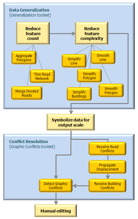
It is important to understand that most geoprocessing tools typically generate new data as an output that can then be used as input for subsequent tools. In contrast to this, cartographers typically follow a workflow that is characterized by incremental improvement of feature layers already established in a map document. Symbology, layer properties, and masking relationships are already defined, so it follows that it is preferable to modify input layers as conflict resolution and generalization operations are performed so as not to lose this information. For this reason, some of the tools in the Cartography toolbox modify input data in symbolized layers rather than creating data. This approach is particularly manageable and powerful when used in conjunction with cartographic representations.
Using representations to support generalization
Representations are a property of geodatabase feature classes that can support an alternate display of the feature geometry. Feature classes can have multiple representations associated with them, thereby supporting multiple displays of the same data. Representations play an advantageous role in generalization, but it must be understood that a single feature class is created for a specific scale (or small range of scales) regardless of how many representations are associated with it. It may seem that being able to use representations to support multiple displays of a set of features means that representations can be used to draw the same features at different scales. Some small changes in scale can be accomplished gracefully by making some minor adjustments to the shapes of some representation features or even by hiding some. But there is still a one-to-one relationship maintained even with representations; each feature can have one or more alternate displays, but features cannot be combined into new features. For example, a set of discrete buildings cannot be modeled as a built-up area using representation display alone. To truly support multiscale mapping, features must be processed appropriately to ensure sensible feature density and detail and to avoid symbolized conflicts. The tools found in the Generalization and Graphic Conflicts toolsets can help you accomplish this.
Learn more about conflict resolution and generalization
Representations have one of two editing behavior settings. The editing setting is a property of a representation and is established when a representation is created on a feature class. 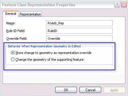
- Store change to geometry as representation override—This is the default setting. It means that modifications to the geometry of features will be stored in a separate BLOB field in the feature class attribute table, which is only accessible by the current representation. The base geometry of the feature stored in the Shape field is left intact.
- Change the geometry of the supporting feature—With this setting, modifications to the geometry of features will modify the actual Shape field of the feature class, impacting any other representations associated with the feature class.
Some of the generalization tools modify their input layers; new datasets are not created. This is called in/out derived data. It is strongly recommended that you use layers pointing to representations with the Store change to geometry as representation override setting, especially when working with the graphic conflict tools (Resolve Road Conflicts, Propagate Displacement, or Resolve Building Conflicts), because these tools modify the geometry of the input layers. With this setting, the modifications made to features by these tools will be stored as overrides in the representation, and the original geometry is unchanged. The advantage of working in this way is that the original shapes of features are readily available (in the Shape field) to visually compare or even revert to if results are not suitable.
Representations are also advantageous when generalizing data across a fairly large-scale range. Ideally, generalization processes should be able to handle large reductions in scale directly, but an intermediate scale is usually necessary. Preparing data for display at intermediate scales to bridge the transition can exaggerate inaccuracies, because different decisions should be made as detailed data drops from the display. For example, consider feature A displaced to accommodate feature B on large-scale map. On smaller-scale map, feature B no longer appears, but there is no easy way to see that A has been displaced or determine where it came from. In this case, a now-unnecessary inaccuracy is propagated to the next smaller scale. Representation overrides help this situation, because you can quickly and easily visually determine the starting location of a feature and revert to it as necessary.
Chaining generalization tools in ModelBuilder
Generalization tools make use of multivalue inputs—that is, a list of one or more feature classes. Many geoprocessing tools accept multiple values (such as the Union tool), but generalization tools are a bit unusual in that they also output multivalues. This requires that you be aware of a few ModelBuilder techniques to produce the model you want. These techniques are discussed below.
Chaining tools with multiple inputs and outputs
The Thin Road Network, Resolve Road Conflicts, and Resolve Building Conflicts tools output multivalues. This means that only tools that accept multivalue inputs can use the output of these tools directly. For example, if three layers are used as inputs to the Thin Road Network tool, and you want to use these same three layers as inputs into the Resolve Road Conflict tool after they have been thinned, you can chain the output of the Thin Road Network tool directly to the Resolve Road Conflicts tool.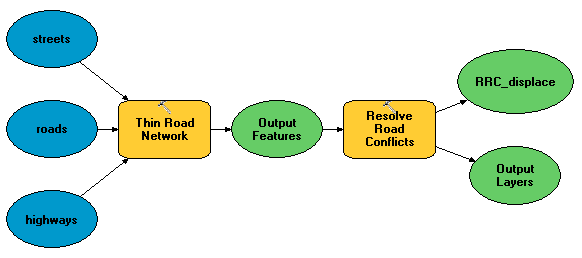
You can use the Collect Values tool to add more layers to a multivalue. The example below shows adding two more layers to the output of Thin Road Network to create the input to Resolve Road Conflicts.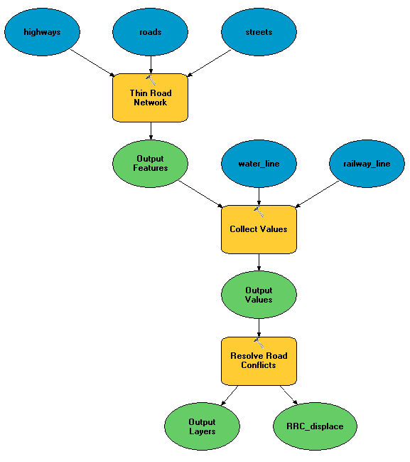
Chaining multiple outputs to a single input
To chain tools that have a multivalue output to a tool that accepts a single input, use the Append tool to merge multiple feature
classes together. An example of this workflow is appending
multiple road input layers that were processed by the Thin Road Network tool to use as an input to the Merge Divided Roads tool, which accepts only a single input.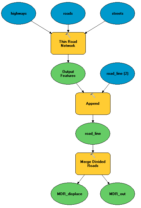
Chaining multiple inputs individually
In some cases, you want to pass multiple outputs from a tool individually to another tool. This would be the case if you didn't want all the outputs from the first tool to participate in the second tool, or if you wanted to set specific parameters for each input in the second tool. For example, the Resolve Building Conflicts tool allows full control over the way each input layer is defined as a barrier. In these cases, use the same set of layers as inputs to both tools, but set the output of the first tool as a precondition to the second tool to enforce the correct order of processing, as illustrated below. This approach is only applicable when the first tool, like the Resolve Road Conflicts tool, modifies input layers instead of creating new output layers.
Learn more about using preconditions in ModelBuilder
In the example below, the three transportation layers are used as inputs to both tools. This is possible because these layers are modified by the Resolve Road Conflicts tool; new output feature classes are not created. The output of the Resolve Road Conflicts tool is used as a precondition to the processing of the Resolve Building Conflicts tool to ensure that the Resolve Road Conflicts tool completes processing before the Resolve Building Conflicts tool begins. 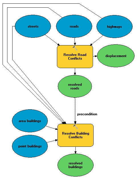
Symbolized inputs
To chain tools that only accept symbolized layers, you will need to use the Make Feature Layer tool and the Apply Symbology From Layer tool to prepare an output layer for chaining purposes in ModelBuilder as well as in scripting environments. 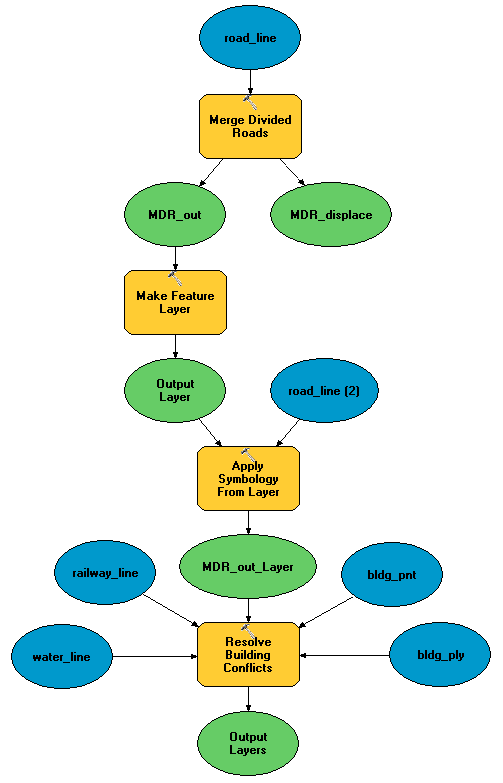
A sample Python script to prepare data for display at a smaller scale
Cartography toolbox workflow example (stand-alone script)
This stand-alone script goes through a sample workflow using a number of tools from the Cartography toolbox to generalize 1:25,000-scale data and resolve graphical conflicts to display at 1:50,000 scale.
# Name: cartography_workflow_script.py
# Description: Process features in order to resolve graphic conflicts when
# changing scales from 25K to 50K.
#
# Tools used = Aggregate Polygons, Align Marker To Stroke Or Fill, Apply
#              Symbology From Layer, Create Overpass, Create Underpass, Calculate
#              Line Caps, Eliminate Polygon Part, Make Feature Layer, Merge
#              Divided Roads, Propagate Displacement, Resolve Building Conflicts
#              Resolve Road Conflicts, Select, Select Layer By Attribute, Set
#              Representation Control Point At Intersect, Set Representation
#              Control Point By Angle, Simplify Building,Simplify Line, Simplify
#              Polygon, Smooth Line, Smooth Polygon, Thin Road Network
# Minimum ArcGIS version = 10
# Author: ESRI
#
# The geodatabase used in this workflow is assumed to be in c:\data
# - please replace this path to your machine specific folder.


# Import system modules
import arcpy, sys, os
from arcpy import env

# Start the processing
env.workspace = "C:/data/cartography.gdb"

# The data was captured at a scale of 1:24000, and this workflow will produce
# data appropriate for a scale of 1:50000.
# Most of the geoprocessing tools in this workflow require a reference scale
env.referenceScale = "50000"
env.cartographicCoordinateSystem = ""


###############
# HYDROGRAPHY #
###############

# A subset of linear features (rivers/streams) will be processed
# for simplification and smoothing
# A subset of polygonal features (reservoirs/lakes) will be procesed
# for simplification and smoothing

# The workspace is set to the hydrography feature dataset
env.workspace = "C:/data/cartography.gdb/hydrography"

# Linear hydrographic features
arcpy.MakeFeatureLayer_management("streamnetwork", "streamlayer", "", "", "")

# A selection is made for features which are rivers/streams
arcpy.SelectLayerByAttribute_management("streamlayer", "NEW_SELECTION",
                                        '"FCsubtype" = 1')

# In order to reduce the complexity from the streams, vertices are removed using
# the Simplify Line tool
arcpy.SimplifyLine_cartography("streamlayer", "streams_simplified",
                               "BEND_SIMPLIFY", "100 meters", "RESOLVE_ERRORS")

# In order to reduce the amount or severity of sharp angles, Smooth Line is used
# to improve the shape of the streams
arcpy.SmoothLine_cartography("streams_simplified", "streams",
                             "BEZIER_INTERPOLATION", "#", "0", 'FLAG_ERRORS')

# Some of the processed features are intermittent rivers or streams and are
# symbolized as dashed lines. When symbolized with representations, the dashes
# can be centered around corners to improve the look of the features. The corners
# are identified as vertices which will be flagged as representation control
# points. Representation symbology is applied to a feature layer in order to be
# processed for control points.

# To place dashes at corners, representation symbology needs to be used by
# the feature layer.
arcpy.MakeFeatureLayer_management("streams", "streamslayer", "", "", "")

# Representation symbology is applied to a feature layer in order to be
# processed for control points.
arcpy.ApplySymbologyFromLayer_management("streamslayer",
                                         "C:/data/stream_symbols.lyr")

# The dashes in the stream symbol will be placed at control points created
# anywhere an angle is less than (or equal to) 130 degrees.
arcpy.SetRepresentationControlPointByAngle_cartography("streamslayer", "130")

# Polygonal hydrographic features
# A selection is made to create a new feature class for reservoirs.
arcpy.Select_analysis("openwater", "reservoirs", '"FCsubtype" = 4')

# A selection is made to create a separate feature class for processing in order
# to generate lakes.
arcpy.Select_analysis("openwater", "water_select", '"FCsubtype" <> 4')

# In order to reduce the complexity from the lakes, vertices are removed using
# the Simplify Line tool.
arcpy.SimplifyPolygon_cartography("water_select", "water_simplified",
                                  "BEND_SIMPLIFY", "100 meters", "0",
                                  "RESOLVE_ERRORS")

# In order to reduce the amount (or severity) of sharp angles, Smooth Line is
# used to improve the shape of the lakes.
arcpy.SmoothPolygon_cartography("water_simplified", "lakes",
                                "BEZIER_INTERPOLATION", "0", "", "FLAG_ERRORS")


#############
# RAILROADS #
#############

# Set the workspace to the transportation feature dataset
env.workspace = "C:/data/cartography.gdb/transportation"
# In order to reduce the complexity from the railroads, vertices are removed
# using the Simplify Line tool.
arcpy.SimplifyLine_cartography("railnetwork", "rail_simplified",
                               "BEND_SIMPLIFY", "100 meters", "RESOLVE_ERRORS")

# The Merge Divided Roads tool requires symbolized features, so pre-made
# symbology is provided to the feature layer.
arcpy.MakeFeatureLayer_management("rail_simplified", "railwaylayer", "", "", "")

# In this workflow, the symbology being applied is Representations
arcpy.ApplySymbologyFromLayer_management("railwaylayer",
                                         "C:/data/rail_symbols.lyr")

# The Merge Divided Roads tool will be used to generates single line railroad
# features in place of multiple divided railroad lanes.
arcpy.MergeDividedRoads_cartography("railwaylayer", "level", "25 Meters",
                                    "railways")

# To place markers at corners, representation symbology needs to be used by
# the feature layer.
arcpy.MakeFeatureLayer_management("railways", "railwayslayer", "", "", "")

# Representation symbology is applied to a feature layer in order to be
# processed for control points.
arcpy.ApplySymbologyFromLayer_management("railwayslayer",
                                         "C:/data/rail_symbols.lyr")

# The tick marks in railroad symbol (markers) will be placed at control points
# created anywhere an angle is less than (or equal to) 130 degrees.
arcpy.SetRepresentationControlPointByAngle_cartography("railwayslayer", "130")


###########
# LANDUSE #
###########

# Set the workspace to the landuse feature dataset
env.workspace = "C:/data/cartography.gdb/landuse"
# The polygons which represent landcover have holes in them where buildings are
# located. The holes need to be removed so they will not appear after buildings
# have moved. In this example, any hole which is less than 50 percent of the
# feature's area will be removed.
arcpy.EliminatePolygonPart_management("cultural", "urban_area", "PERCENT", "0",
                                      "50", "CONTAINED_ONLY")


##############
# BOUNDARIES #
##############

# The boundary features have dashed outlines which are not in phase with each
# other on shared edges between features. To make the dashed outlines in phase
# with each other, representation control points are added wherever features
# share coincident vertices. The control points are then added to the features
# symbolized with Representations.
arcpy.SetRepresentationControlPointAtIntersect_cartography
("C:/data/boundaries.lyr", "C:/data/boundaries.lyr")


#########
# ROADS #
#########

# Set the workspace to the transportation feature dataset
env.workspace = "C:/data/cartography.gdb/transportation"
# Linear features

# Roads which are dead ends (or cul-de-sacs) should have their Line ending
# property set to BUTT.
arcpy.CalculateLineCaps_cartography("C:/data/road_symbols.lyr", "BUTT",
                                    "CASED_LINE_DANGLE")

# Thin Road Network identifies a subset of road segments that can be removed from
# the display to create a simplified road network that retains the connectivity
# and general character of the input collection. Features are flagged for removal
# when their attribute value in the "invisible" field equals one. A layer
# definition query can be used to display the resulting simplified feature class.
arcpy.ThinRoadNetwork_cartography("roadnetwork", "500 meters", "invisible",
                                  "level")

# The Merge Divided Roads tool will be used to generates single line road
# features in place of multiple divided road lanes.
arcpy.MergeDividedRoads_cartography("C:/data/road_symbols.lyr", "level",
                                    "25 meters", "roads")

# The Resolve Road Conflicts tool requires symbolized features, so pre-made
# symbology is provided to the feature layer.
arcpy.MakeFeatureLayer_management("roads", "roadslayer", "", "", "")

# In this workflow, the symbology being applied is Representations
arcpy.ApplySymbologyFromLayer_management("roadslayer",
                                         "C:/data/road_symbols.lyr")

# The Resolve Road Conflicts tool does not produce output road layers but instead
# alters the source feature classes of the input road layers. The Resolve Road
# Conflicts tool adjusts line features to ensure that they are graphically
# distinguishable when symbolized at output scale.
arcpy.ResolveRoadConflicts_cartography
("roadslayer", "level", "C:/data/cartography.gdb/buildings/displacement")

# The dashes in the road symbols will be placed at control points created
# anywhere an angle is less than (or equal to) 130 degrees.
arcpy.SetRepresentationControlPointByAngle_cartography("roadslayer", "130")

# Create bridges
# The Create Overpass tool will create a bridge for the roads and a mask for the
# streams wherever a road goes over a steam.
arcpy.CreateOverpass_cartography("roadslayer", "streamslayer", "2 points",
                                 "1 points", "over_mask_fc", "over_mask_rc",
                                 '"BridgeCategory" = 1', "bridges",
                                 "ANGLED", "1 points")

# Create tunnels
# The Create Overpass tool will create a tunnel for the railroads and a mask for
# the railroads wherever a railroad goes under a road.
arcpy.CreateUnderpass_cartography("roadslayer", "railwayslayer", "2 points",
                                  "1 points", "under_mask_fc", "under_mask_rc",
                                  '"RelationshipToSurface" = 3', "tunnels",
                                  "ANGLED", "1 points")


#############
# BUILDINGS #
#############

# Set the workspace to the buildings feature dataset
env.workspace = "C:/data/cartography.gdb/buildings"
# Point features

# When the road features were adjusted by the Resolve Road Conflicts tool, the
# spatial relationship with nearby buildings was affected. A displacement feature
# class was created by that tool in order to record the change applied to the
# roads. This information can be used by the Propagate Displacement tool to apply
# the same change to the point buildings.

# The road displacement is propagated to the point buildings
arcpy.PropagateDisplacement_cartography("point_bldg", "displacement", "AUTO")

# Point buildings will be rotated against nearby linear roads
# The Align Markers To Stroke Or Fill tool can do this with features symbolized
# with Representations.

# A feature layer is made for point buildings
arcpy.MakeFeatureLayer_management("point_bldg", "bldglayer", "", "", "")

# The symbology is switched to Representations
arcpy.ApplySymbologyFromLayer_management("bldglayer", "C:/data/bldg_symbols.lyr")

# The Align Marker to Stroke Or Fill tool is used to align point buildings to
# face road features within 5 points of the buildings
arcpy.AlignMarkerToStrokeOrFill_cartography("bldglayer", "roadslayer",
                                            "5 points", "PERPENDICULAR")

# Polgyonal features
# When the road features were adjusted by the Resolve Road Conflicts tool, the
# spatial relationship with nearby buildings was affected. A displacement
# feature class was created by that tool in order to record the change applied
# to the roads. This information can be used by the Propagate Displacement tool
# to apply the same change to the polygonal buildings.

# The road displacement is propagated to polygon buildings
arcpy.PropagateDisplacement_cartography("footprints", "displacement", "SOLID")

# A selection is made to create a feature class with buildings larger than
# a minimum size
# The small buildings are not appropriate at the new map scale of 1:50,000
arcpy.Select_analysis("footprints", "buildings_select", '"Shape_Area" > 100')

# There is a need to create better spacing between polygon buildings and combine
# them when they share edges or are very close together
# The Aggregate Polygons tool is used to accomplish this task
arcpy.AggregatePolygons_cartography("buildings_select", "large_buildings",
                                    "20 meters", "", "", "ORTHOGONAL")

# In order to reduce the complexity of the buildings, indentations, extensions
# and extra vertices are removed using the Simplify Building tool.
# Buildings require less visible detail at the new scale of 1:50,000.
arcpy.SimplifyBuilding_cartography("large_buildings", "area_bldg", "20 meters",
                                   "0 unknown", "CHECK_CONFLICTS")

# All buildings require further improvements to achieve better spacing between
# themselves and other nearby features. At the new scale of 1:50,000 the
# symbolized buildings may overlap other features and create a visually congested
# map. To improve the visual congestion, the Resolve Building Conflicts tool is
# used. Buildings are improved in the context of their surrounding features.
# These features are considered barriers to buildings. The Resolve Building
# Conflicts tool requires symbolized features and has several options available
# to improve the buildings. Options include: moving or resizing the buildings,
# orienting or snapping the buildings to nearby features, as well as making the
# buildings invisible. Buildings from multiple feature classes can be used as
# inputs to the tool. Barriers from multiple feature classes can be used as
# inputs to the tool. For each barrier, the option is available to specify a snap
# or orient action for the buildings when they are within a specified distance.
# For each barrier, the option is available to specify a minimum distance for
# buildings to maintain between them.

# A feature layer is made for the polygon buildings
arcpy.MakeFeatureLayer_management("area_bldg", "footprintlayer", "", "", "")

# The symbology is switched to Representations
arcpy.ApplySymbologyFromLayer_management("footprintlayer",
                                         "C:/data/footprint_symbols.lyr")

# The Resolve Building Conflicts tool is run with point and polygon buildings
# against roads, streams and railroads. The buildings will be moved away from
# streams and railroads until they reach a minimum distance. The buildings
# within a maximum distance from the roads will be rotated. Further movement
# and rotation may still be required by the tool in order to resolve any
# remaining graphic conflict.
arcpy.ResolveBuildingConflicts_cartography("footprintlayer; bldglayer", "invisible",
                                           "'roadslayer' 'true' '5 meters';'streamslayer' 'false' '5 meters';'railwayslayer' 'false' '10 meters'",
                                           "10 meters", "20 meters", "level")