Description
The Transform tool converts data from one coordinate system to another. It is often used to convert coverages created in digitizer units (most often inches) to the real-world units represented on the map manuscript. These real-world locations are represented by a particular projection; for example, the projection of your basemap may be UTM with control point locations measured in meters.
To perform a transformation, you must be able to register at least two tics in your coverage to real locations. These real locations may be measured in feet or meters using the basemap coordinate system, or they may be located at latitude-longitude intersections. If your locations reference degrees of latitude and longitude, use the Project tool to convert the control points to the coordinate system that corresponds to your base map, measured in feet or meters. Do this before transforming the digitized coverage.
When you initially transform your data, you will be transforming it into the same projection as your source map. You can then use Project tool to convert the coverage to another map projection.
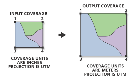
The Transform tool is based on comparing the coordinates of the Input Coverage's tics with the coordinates for corresponding tics in the Output Coverage. The Tic-IDs identify the tics to be compared. The minimum number of needed tics depends on which transformation option is used. Tics are treated as control points for the transformation, and they are not converted with the transformation equation. The coordinates of the output tics will not change after the transformation. However, any features that coincide with the input tics usually will not coincide with the output tics. You may need to adjust features to force them to coincide with the tics in the Output Coverage after the transformation.
The Transform tool, by default, uses an AFFINE transformation function to transform coverage coordinates from the Input Coverage to the Output Coverage. A minimum of three tics is required to calculate an affine transformation.
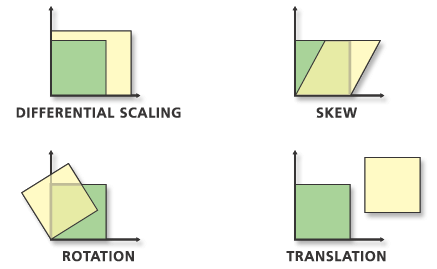
An affine transformation can differentially scale the data, skew it, rotate it, and translate it. The graphic below illustrates the four possible changes.
The affine transformation function is:
x’ = Ax + By + CThe parameters A-F are determined by the control points,
y’ = Dx + Ey + Fthen applied to all coordinates in the coverage.
where x and y are coordinates of the Input Coverage, and x' and y' are coordinates of the Output Coverage. A, B, C, D, E, and F are determined by comparing the location of tics in the Input Coverage and their locations in the Output Coverage. They scale, skew, rotate, and translate the tic coordinates.
The Transform tool reports the six parameters and their geometric interpretation. Here is an example of part of the output report for an affine transformation.
Transforming coordinates for coverage in_cov_name
Scale (X,Y) = (246.140,255.702)  Skew (degrees) = (-0.061)
Rotation (degrees) = (0.334)  Translation = (2890.267,3679.906)
RMS Error (input, output) = (0.084,20.592)

Affine X = Ax + By + C
       Y = Dx + Ey + F
A =   246.135   B =   -1.763        C =   2890.267
D =   1.434     E =   255.696       F =   3679.906
One section of the report lists the parameters of the transformation equations. You can interpret the equation parameters to understand what is happening geometrically. The first section of the report gives the interpreted values of the scaling, skewing, and rotation. Rearranging the order of the application of these geometric actions changes their interpreted values, but the final result and the equation parameters are always the same. The interpretation used is in the order of (1) scaling, (2) skewing in the x direction, and (3) counterclockwise rotation of points around the axes. The translation values are not interpreted but are simply the C and F translation parameters from the equations. The Transform tool interprets the affine equation parameters in the following manner:
A = mx · cos t
B = my · (k · cos t - sin t)
D = mx · sin t
E = my · (k · sin t + cos t)
C = translation in x direction
F = translation in y direction

where

mx = change of scale in x direction
my = change of scale in y direction
k = shear factor along the x-axis = tan (skew angle) (the skew angle is measured from the y-axis)
t = rotation angle, measured counterclockwise from the x-axis
The rotation angle refers to the rotation of the data about a fixed x,y coordinate system. Referring to the earlier figure, the original data has been rotated 45 degrees. A negative value means the data is rotated clockwise from the x-axis.
The SIMILARITY transformation scales, rotates, and translates the data. It will not independently scale the axes nor introduce any skew. A similarity transformation requires a minimum of two control points. Here's the report for a similarity transformation using the same coverages previously transformed with an affine transformation.
Transforming coordinates for coverage in_cov_name
Scale (X,Y) = (249.927,249.927)
Rotation (degrees) = (0.362)  Translation = (2855.407,3715.168)
RMS Error (input, output) = (0.118,29.398)

Similarity X =  Ax + By + C
           Y = -Bx + Ay + F
A =   249.922         B =   -1.578
C =   2855.407        F =   3715.168
Notice that the X and Y scale values are equal. A skew value is not reported because the similarity transformation will not allow any nonorthogonal movement to be introduced into the data.
The similarity transformation function is
x’ =  Ax + By + C
y’ = -Bx + Ay + F

where

A = s · cos t
B = s · sin t
C = translation in x direction
F = translation in y direction

and

s = scale change (same in x and y directions)
t = rotation angle, measured counterclockwise from the x-axis
Just as in the AFFINE explanation, the rotation angle refers to the rotation of the data about a fixed x,y coordinate system. Referring to the earlier figure, the original data has been rotated 45 degrees. A negative value means the data is rotated clockwise as measured from the x-axis.
The PROJECTIVE transformation is based upon a more complex formula which requires a minimum of four tics.
x’ = (Ax + By + C) / (Gx + Hy + 1)
y’ = (Dx + Ey + F) / (Gx + Hy + 1)
The PROJECTIVE report includes the approximate scale, the RMS error, and the equation parameters. Due to the complexity of the interpretation, the projective transformation parameters are not interpreted. For more information, please refer to one of the photogrammetric texts listed in the references at the end of this topic. Below is a sample output report for a projective transformation.
Transforming coordinates for coverage in_cov_name
Approximate scale = 1479.087
RMS Error (input, output) = (0.040,60.878)

2D Projective  X = (Ax + By + C) / (Gx + Hy + 1)
               Y = (Dx + Ey + F) / (Gx + Hy + 1)

A =         55.667   B =       -718.999   C =    2125052.558
D =       -199.525   E =       1385.541   F =     317759.475
G =         -0.001   H =          0.000

Principal point of input (xp,yp) = (2.000,16.946)
Exposure center of output(Xc,Yc) = (2127791.000,343183.000)
The principal point and exposure center correspond to the first tic in the Input Coverage tic file. If you want to use another point (for instance, the center of the dataset), make sure it is the first tic in the file.
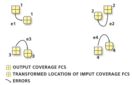
A Root Mean Square (RMS) error is calculated for each transformation performed and indicates how good the derived transformation is. The following example illustrates the relative location of four output control points (tics) and the transformed input control points:
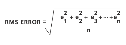
The RMS error measures the errors between the Output Coverage's tics and the transformed locations of the Input Coverage's tics.
The transformation is derived using least squares, so more tics than necessary can be given.
The RMS error for each transformation is reported in both Input Coverage units (for example, 0.031 inches) and Output Coverage units (for example, 37.465 feet).
RMS Error (input, output) = (0.031,37.465)A perfect transformation produces an RMS error of zero. Although you will not obtain a value of 0.000, you should try to keep your RMS error as low as possible. It is best to establish and maintain a maximum acceptable error. Acceptable values will vary depending on the accuracy of the original data and the scale of the source map. High RMS errors indicate that the old tics and the new tics do not correspond to the same relative locations. If your RMS error is higher than the established value, it can indicate conversion problems that may incorrectly stretch your Output Coverage.
The last part of the report lists the input and output tic coordinates and their x and y errors (see below). The transformation parameters are a best fit between the input and output tics. If you use the transformation parameters to transform the actual input tics, the transformed output locations won't match the true output tic locations. The x and y errors are a measure of the fit between the true locations and the transformed locations of the output tics. Sometimes you can spot a mistake by looking at the x and y errors.
tic id  input x   input y   output x      output y     x error   y error
------------------------------------------------------------------------
1       2.000     16.946    2127791.000   343183.000    14.463    75.499
2       12.764    16.821    2143469.000   343326.000   -31.043   -85.363
3       2.052     1.976     2128000.000   320680.000   -36.290    -2.353
4       12.922    2.013     2143729.000   320912.000    20.245    -6.163
5       2.082     9.442     2127944.000   332015.000    22.016   -74.699
6       12.662    9.442     2143320.000   332015.000    10.609    93.079
Example
This example transforms a coverage from digitizer units to real-world coordinates. The original coverage named INCHCOV has the following control points measured in digitizer inches:
IDTIC    XTIC       YTIC
1       2.000     16.946
2      12.764     16.821
3       2.052      1.976
4      12.922      2.013
5       2.082      9.442
6      12.662      9.442
The basemap used was in the State Plane coordinate system with control points measured in feet. Each tic corresponds to the following locations:
Tic-IDs	 X Coordinates	 Y Coordinates
1	       2,127,791     	343,183
2       	2,143,469     	343,326
3       	2,128,000     	320,680
4       	2,143,729     	320,912
5       	2,127,944     	332,015
6	       2,143,320     	332,015
The Output Coverage must exist before the Transform tool can be executed. Use the Create Coverage tool to create the Output Coverage and copy the TIC and BND files from the Input Coverage if desired. Optionally, you can use the Generate tool to create a new coverage containing tics in the desired locations.
The tic file for the Output Coverage must contain x,y coordinates for each tic to be retained in the Output Coverage; in this case, the tic locations in the State Plane coordinate system. Tic coordinates can be adjusted in ArcMap or in ArcInfo Workstation TABLES or INFO modules.
Once the new tics have been created, the features in the digitized coverage can be transformed to real-world units. The Transform tool is used to convert a State Plane projection coverage referenced in inches (INCHCOV) to a State Plane projection coverage referenced in feet (STATECOV). Here is an example of the AFFINE transformation.
Scale (X,Y) = (1452.317,1508.433)  Skew (degrees) = (0.416)
Rotation (degrees) = (0.218) Translation = (2124994.654,317664.385)
RMS Error (input, output) = (0.048,71.614)

Affine  X = Ax + By + C
        Y = Dx + Ey + F
A =     1452.230   B =       -5.526   C =   2124994.654
D =       15.858   E =     1508.462   F =    317664.385

tic id  input  x      input  y
        output x      output y   x error   y error
--------------------------------------------------
1          2.000        16.946
     2127791.000    343183.000    14.463    75.499
2         12.764        16.821
     2143469.000    343326.000   -31.043   -85.363
3          2.052         1.976
     2128000.000    320680.000   -36.290    -2.353
4         12.922         2.013
     2143729.000    320912.000    20.245    -6.163
5          2.082         9.442
     2127944.000    332015.000    22.016   -74.699
6         12.662         9.442
     2143320.000    332015.000    10.609    93.079
Here is the corresponding example of a PROJECTIVE transformation for the same coverage. Remember that the PROJECTIVE option is normally used only when the original coverages are digitized directly from aerial photos.
Transforming coordinates for coverage INCHCOV
Approximate scale = 1479.087
RMS Error (input, output) = (0.040,60.878)

2D Projective  X = (Ax + By + C) / (Gx + Hy + 1)
               Y = (Dx + Ey + F) / (Gx + Hy + 1)
A =         55.667   B =       -718.999   C =    2125052.558
D =       -199.525   E =       1385.541   F =     317759.475
G =         -0.001   H =          0.000

Principal point of input (xp,yp) = (2.000,16.946)
Exposure center of output(Xc,Yc) = (2127791.000,343183.000)

tic id  input  x      input  y
        output x      output y   x error   y error
--------------------------------------------------
1         2.000         16.946
    2127791.000     343183.000    -4.438    45.252
2        12.764         16.821
   2143469.000      343326.000   -11.447   -36.202
3         2.052          1.976
   2128000.000      320680.000   -17.300    46.421
4        12.922          2.013
   2143729.000      320912.000     1.704   -36.962
5         2.082          9.442
   2127944.000      332015.000    21.787   -93.410
6        12.662          9.442
   2143320.000      332015.000     9.694    74.901
Finally, here is the same coverage transformed using the SIMILARITY option.
Transforming coordinates for coverage inchcov
Scale (X,Y) = (1483.794,1483.794)
Rotation (degrees) = (0.377)  Translation = (2124800.900,317942.729)
RMS Error (input,output) = (0.162,240.958)

Similarity  X =  Ax + By + C
Y = -Bx + Ay + F
A =         1483.762   B =           -9.765
C =      2124800.900   F =       317942.729

tic id  input  x      input  y
        output x      output y   x error   y error
--------------------------------------------------
1          2.000        16.946
     2127791.000    343183.000  -188.053   -76.916
2         12.764        16.821
     2143469.000    343326.000   106.378  -300.277
3          2.052         1.976
     2128000.000    320680.000  -173.717   214.680
4         12.922         2.013
     2143729.000    320912.000   225.411   143.724
5          2.082         9.442
     2127944.000    332015.000  -146.109   -42.262
6         12.662         9.442
     2143320.000    332015.000   176.089    61.051
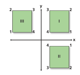
The following example flips a coverage using an AFFINE transformation.
Transforming coordinates for coverage flag
Scale (X,Y) = (1.000,-1.000)  Skew (degrees) = (0.000)
*** Negative Y scaling indicates reflection around X axis. ***
Rotation (degrees) = (180.000)  Translation = (800.000,0.000)
RMS Error (input, output) = (0.000,0.000)

Affine  X = Ax + By + C
        Y = Dx + Ey + F
A =       -1.000   B =        0.000   C =      800.000
D =        0.000   E =        1.000   F =        0.000

tic id  input  x      input  y
        output x      output y   x error   y error
--------------------------------------------------
1        700.000      100.000
         100.000      100.000      0.000     0.000
2        700.000      800.000
         100.000      800.000      0.000     0.000
3        100.000      800.000
         700.000      800.000      0.000     0.000
4        100.000      100.000
         700.000      100.000      0.000     0.000
Note the message in the output report about the reflection. What is happening to the coverage is shown in the graphic below. The rectangle labeled I is the Input Coverage. A Y scale of -1 is applied to the coordinates. This results in the II rectangle. There is no skew factor, so the points are rotated 180 degrees, which places it in position III. The final step (not shown) is to translate the coverage.
References
Maling, D.H., Coordinate Systems and Map Projections. George Philip., 1973.
Maling, D.H., “Coordinate systems and map projections for GIS.” In: Maguire D.J., M.F. Goodchild, and D.W. Rhind (eds.), Geographical Information Systems: principles and applications. Vol. 1, pp. 135-146. Longman Group UK Ltd., 1991.
Moffitt, F.H., and E.M. Mikhail, Photogrammetry. Third Edition. Harper and Row, Inc., 1980.
Pettofrezzo, A.J., Matrices and Transformations. Dover Publications, Inc., 1966.
Slama, C.C., C. Theurer, and S.W. Henriksen (eds.), Manual of Photogrammetry. 4th Edition. Chapter XIV, pp. 729-731. ASPRS, 1980.