The following are the available distributions to a variety of tools that create random values. The distributions transform the 0–1 random values created from the specified stream (identified either globally in the analysis environment or locally to the tool) into the specified distribution. See The distribution syntax for random values for the syntax and parameters for each distribution.
Uniform distribution
Uniform distribution is a continuous probability distribution in which all values within a specified interval have the same probability. An integer distribution is a discrete version of uniform distribution (see below). Uniform distribution can be used when modeling concentrations of a gas in a simulation model or the time between accidents at an intersection, as well as for placing the points in the Create Random Points tool.
Uniform distribution is often used to model random events when each potential outcome or occurrence has equal probability of occurring.
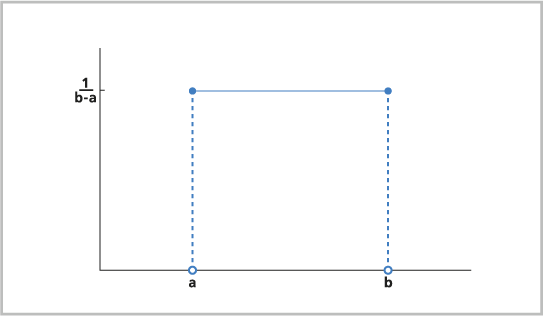
The formula for uniform distribution is as follows:

where
a is the minimum value for the interval with equal probability.
b is the maximum value for the interval with equal probability.
x is the observations.
The random values selected are between the minimum and maximum (both exclusive). The minimum must be less than the maximum. If no minimum and maximum are provided, uniform variables between 0.0 and 1.0 are produced.
Integer distribution
Integer distribution is a probability distribution in which all discrete values within a specified interval have the same probability. Integer distribution is the discrete version of uniform distribution (see above). Integer distribution can be used to model the chance of each number occurring when throwing a die (each number has a one-sixth probability of occurring), modeling random events in a simulation model, or selecting sampling locations for a biological study.
Integer distribution is used often to model random events when each potential outcome or occurrence has equal probability of occurring.
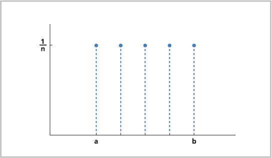
The formula for the integer distribution is shown here:

where
a is the minimum value for the interval with equal probability.
b is the maximum value for the interval with equal probability.
x is the observations.
The random values selected are between the minimum and maximum (both exclusive). The minimum must be less than the maximum. If no minimum and maximum are provided, uniform values between 1 and 100 are produced.
Normal distribution
Normal distribution models continuous random variables that commonly occur. Normal distribution is widely used and is applicable in many applications. It is built on the central limit theorem, which is based on the principle that the sum of the random variables is normally distributed if there are a large number of observations. For example, the number of times heads appears in a sequence of coin flips will approach normality if the coin is flipped many times. Examples of normal distributions are height of people in a country, elevation values in a state, and math test scores for all 12-year-old students.
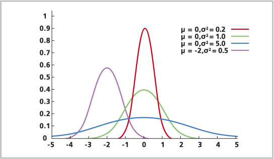
The formula for normal distribution is as follows:

where
μ is the mean.
σ is the standard deviation (a positive number).
Normal distribution is symmetrical relative to the mean, mode, and median, which are all equal at μ.
Often binomial and Poisson distributions model future discrete, independent, random, true, or false events (for example, the number of times heads appears when flipping a coin) using a relatively small number of observations, while the normal distribution models continuous variables (for example, height, weight, and amount) using a large number of observations. Binomial and Poisson distributions are based on probability, while normal distribution is the number of observations meeting the amount or magnitude.
Exponential distribution
Exponential distribution is a continuous probability distribution. It is generally used to model time between events that occur at a constant average rate, or the distribution can be used to model occurrence of events in a per-unit distance. The time until the next car accident at an intersection, the time between seeing two shooting stars in a night sky, and the distance between potholes on a street are all examples where exponential distribution might be used. With each of these examples, as the time or distance increases, there is an exponentially greater chance for the state to change or the event to occur. The occurrences of the events are independent of one another.
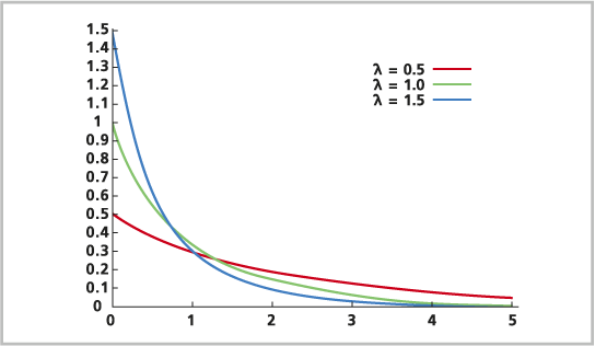
The formula for exponential distribution is as follows:

where
e is the natural logarithm.
x is the possible number of occurrences for the event (positive integer values).
Exponential distribution models Poisson processes where the phenomenon is at an initial state. Exponential distribution is the continuous version of geometric distribution. If the process of moving from state A to state B can be broken into several independent tasks, it might be better to model it with gamma distribution. Gamma distribution models the sum of multiple independent, exponentially distributed variables. It can be viewed as a special case of exponential distribution.
Poisson distribution
Poisson distribution is a discrete probability distribution. Poisson distribution models the probability of the number of events occurring over a fixed time step given a known mean. The events are independent of the last time they occurred. On the x-axis are the discrete values for the events 0, 1, 2, 3, 4, and so on (often representing the number of times the event occurs), and on the y-axis is the probability that the phenomenon occurs that many times given a known mean. The events can be the number of accidents at an intersection, the number of birth defects, or the number of moose in a square kilometer. Poisson distribution models rare occurrences. The distribution is sometimes called the law of small numbers because the event does not happen often, but there are many opportunities for it to occur.
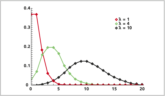
The formula is shown below:

where
e is the natural logarithm.
k is the possible number of occurrences for the event (positive integer values).
k! is a factorial of k.
λ (or the mean) is a positive number representing the expected number of occurrences within a specified interval. If the event occurs every 10 minutes in an hour (60 minutes), the lambda would be 6.
Poisson distribution is similar to binomial distribution; however, Poisson distribution models the occurrence of a rare event without knowing information about the total number of possible occurrences. Poisson distribution examines the number of accidents at an intersection, while binomial models the number of accidents relative to the number of cars passing through the intersection.
Gamma distribution
Gamma distribution is a continuous probability distribution. Gamma distribution models the sum of multiple independent, exponentially distributed variables. It can be viewed as a special case of exponential distribution.
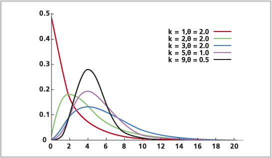
The formula for gamma distribution is as follows:

Another way to parameterize the gamma distribution is shown here:

For an alpha of 1, the gamma distribution equals the exponential distribution. When the alpha is an integer, the gamma distribution becomes the Erlang distribution. For an integer alpha and a beta equaling 2, the gamma distribution becomes a chi-square distribution with 2 alpha degrees of freedom.
The resulting variables are greater than or equal to 0.0. The alpha and beta must be greater than 0.0.
Binomial distribution
Binomial distribution models the number of occurrences of an event when observing a sequence of potential producers of the event. For example, binomial distribution captures the number of people in a clinical study that died of heart disease, the number of people that get off at the second floor in a crowded elevator, or the number of animals in a population that carry a certain genetic trait.
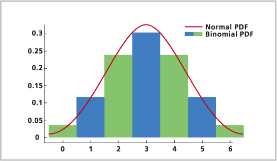
Binomial distribution describes occurrences, not magnitude. It may model how many participants finished a race, not how fast the participants were.
The formula for a binomial distribution is as follows:

where
n is the number of observations.
p is the probability of occurrence.
x is the number of successes ranging from 0 to n.
A common example of the use of binomial distribution is determining the probability of the number of times heads appears when flipping a coin 10 times (n = 10). There can be 0 heads out of 10, 1 out of 10, and so forth; therefore, x = 0, 1, 2, 3, 4, 5, 6, 7, 8, 9, 10. And p is the probability for each x.
All trials are independent, and each trial has an outcome of success or failure.
The Binomial distribution approaches the Poisson distribution for a large n and a small p. In this case, it may be easier to use Poisson distribution.
Binomial distribution returns a random variable for the number of successes out of n trials where the probability for success in each trial is p (for example, the probability of heads turning up is p).
Geometric distribution
Geometric distribution is a discrete probability distribution. There are two main types of phenomena that it models: (1) the probability of the number of times it takes for a success (for example, the number of dice rolls it takes to roll a number 6) or (2) the probability of the number of failures before a success (for example, the number of hikes it takes on a trail before you see a deer). The probability of not seeing a deer on the first hike on the trail is (1 - p). For the second hike, the probability of not seeing a deer is (1 - p) (1 - p). With more hikes on the trail, the probability of not seeing a deer exponentially decreases, and eventually one will be spotted. The events are independent of one another.
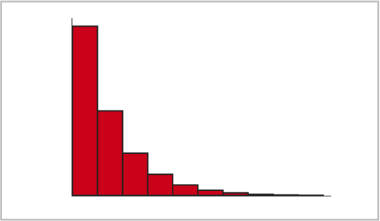
The formula for geometric distribution is as follows:

where
p is the probability of success.
n is the number of trials.
Geometric distribution is the discrete version of exponential distribution (see above). Geometric distribution is a special case of negative binomial or Pascal distribution, with r in the Pascal distribution equaling 1 (see below).
Negative binomial distribution
Negative binomial distribution is a discrete probability distribution. Negative binomial distribution is based on Bernoulli trials. Bernoulli trials model events in which trials have one of two outcomes (success and failure); have a probability of success, p (with p being the same for each trial); and are independent of one another. The flipping of a coin is a Bernoulli trial. For example, negative binomial distribution can model how many flips of a coin it takes until five heads in a row occur. Thus, negative binomial distribution models the number of failures before a success. When r is an integer, the negative binomial becomes a special case known as Pascal distribution.
The formula for negative binomial distribution is as follows:

where
r is the number of failures.
p is the probability of success.
k is the number of successes ranging from 0 to n.
When the negative binomial distribution represents the tossing of a coin, a random value is returned for the number of times it takes for heads to appear.