The Local Outlier Analysis tool identifies significant clusters and outliers in your data. It will find locations in your study area that have been statistically different than their neighbors in both space and time. It takes as input a space-time NetCDF cube created using the Create Space Time Cube By Aggregating Points tool. It then uses the Neighborhood Distance and Neighborhood Time Step parameter values to calculate a space-time implementation of the Anselin Local Moran's I statistic (Cluster and Outlier Analysis) for each bin. To do this, the tool calculates a Local Moran's I index, a pseudo p-value and a type code (CO_TYPE) representing the cluster or outlier category type for each statistically significant bin in the Input Space Time Cube. The pseudo p-values represent the statistical significance of the calculated index values and its precision is dependent on the number of permutations.
Potential applications
Applications for the Local Outlier Analysis tool can be found in many fields, including economics, resource management, political geography, demographics, public health, and fraud prevention. Some of the questions you can answer through the use of this tool include the following:
- Are there locations in my study area with anomalous spending patterns?
- Was there a time period with unexpectedly high rates of disease outbreak across the study area?
- Are there suburban areas where residents are using significantly more water than their neighbors? Or find the suburban areas that use less water consistently to develop best practices for water conservation.
- Are there any locations in my region with significant jumps in the number of insurance claims filed over the last month?
Tool outputs
A number of outputs are created by this tool. The most prominent output is a two-dimensional map summarizing each location over time added to the map upon completion of the tool. The categories are as follows:
| Type Name | Definition |
|---|---|
Never Significant | A location where there has never been a statistically significant CO_TYPE. |
Only High-High Cluster | A location where the only statistically significant type throughout time has been High-High Clusters. |
Only High-Low Outlier | A location where the only statistically significant type throughout time has been High-Low Outliers. |
Only Low-High Outlier | A location where the only statistically significant type throughout time has been Low-High Outliers. |
Only Low-Low Cluster | A location where the only statistically significant type throughout time has been Low-Low Clusters. |
Multiple Types | A location where there has been multiple types of statistically significant cluster and outlier types throughout time (for instance, during some time periods the location has been a Low-High Outlier, and during other time periods it has been a High-High Cluster). |
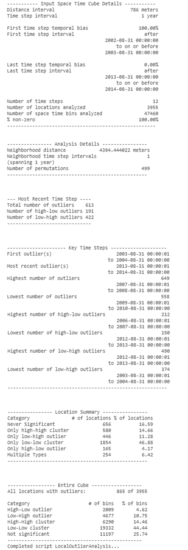
A two-dimensional map summarizing the cluster and outlier types for each location provides the leading output and is added to the map upon completion of the tool. In addition, messages summarizing the analysis results are written to the Results window. Right-clicking the Messages entry in the Results window and selecting View will display the results in a Message dialog box.
These messages include information about the Input Space Time Cube, such as time span, temporal bias, and the number of bins and locations analyzed. It also includes important information about any outliers that occurred in the most recent time step as well as summarizing key time steps that may be of interest. For instance, if your question involves finding underperforming areas in your sales territory and you are looking for low-high outliers, the messages will provide you with the key time step that had the highest number of low-high outliers.

This tool creates a new output feature class with the following fields summarizing the bins at each location of the Input Space Time Cube:
| Alias | Field name |
|---|---|
| Number of Outliers | NUM_OUT |
| Percentage of Outliers | PERC_OUT |
| Number of Low Clusters | N_LOW_CLS |
| Percentage of Low Clusters | P_LOW_CLS |
| Number of Low Outliers | N_LOW_OUT |
| Percentage of Low Outliers | P_LOW_OUT |
| Number of High Clusters | N_HIGH_CLS |
| Percentage of High Clusters | P_HIGH_CLS |
| Number of High Outliers | N_HIGH_OUT |
| Percentage of High Outliers | P_HIGH_OUT |
Locations with No Spatial Neighbors which are relying only on temporal neighbors for analysis calculations | NO_SP_NBR |
Locations with an Outlier in the Most Recent Time Step | OUT_R_TIME |
| Cluster Outlier Type | CO_TYPE |
Additional summary statistics including the sum, minimum value, maximum value, average, standard deviation and median value of the variable analyzed. | SUM_VALUE, MIN_VALUE, MAX_VALUE, MEAN_VALUE, STD_VALUE, and MED_VALUE |
Finally, the Local Outlier Analysis tool adds a number of new variables to your Input Space Time Cube. If these variables already exist (if you run the Local Outlier Analysis tool for the same Analysis Variable multiple times), they will be overwritten so the cube always contains the most recent analysis results.
You may visualize these variables using ArcGIS Pro. See Visualizing the Space Time Cube for strategies.
Interpretation
To aid in the interpretation of the Local Outlier Analysis tool results, the Visualize Space Time Cube in 3D tool can be used to display the result variables added to the cube. The index, p-value, and Cluster Outlier Analysis Type for each bin can be visualized by choosing the Cluster and outlier results Display Theme. An index with a positive value indicates that a bin has neighboring bins with similarly high or low attribute values; this bin is part of a cluster. An index with a negative value indicates that a bin has neighboring bins with dissimilar values; this bin is an outlier. In either instance, the pseudo p-value or p-value for the feature must be small enough for the cluster or outlier to be considered statistically significant. For more information on determining statistical significance, see What is a z-score? What is a p-value?. Note that the Local Moran's I index (I) is a relative measure and can only be interpreted within the context of its generated reference distribution and its computed pseudo p-value or p-value. The pseudo p-value or p-values reported in the output feature class are corrected for multiple testing and spatial dependency.
The cluster or outlier type distinguishes between a statistically significant cluster of high values (High-High), cluster of low values (Low-Low), outlier in which a high value is surrounded primarily by low values (High-Low), and outlier in which a low value is surrounded primarily by high values (Low-High). Statistical significance is set at the 95 percent confidence level. This significance represents an FDR correction, which adjusts the p-value threshold from 0.05 to a value that better reflects the 95 percent confidence level taking into consideration multiple testing.
Neighborhood defaults
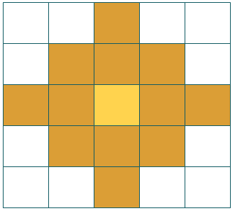
To determine if the bin value at a location in space and time is part of a statistically significant hot or cold spot or a statistically significant outlier, each bin is evaluated within the context of its neighboring space-time bins. The parameter values for Neighborhood Distance and Neighborhood Time Step define the extent of each bin's neighborhood (the context for each bin's analysis). Suppose bin dimensions are 400 meters by 400 meters by 1 day. If you set the Neighborhood Distance to 801 meters and the Neighborhood Time Step to 2, the spatial neighbors will extend two bins both horizontally and vertically, and one bin out diagonally as shown:
In addition, there will be temporal neighbors. All bins at the same location as the target and its spatial neighbors (shown above) for the matching or two preceding time periods—a total of three days, for this example—will be included as neighbors. Notice that temporal neighbors are backward in time only and that a Neighborhood Time Step of 2 encompasses three time-step intervals. To ensure at least 1 temporal neighbor for each location, a Local Moran's Index is not calculated for the bins in the first time slice. The bin values in the first time slice are, however, included in the calculation of the global average.
When you do not provide a value for the Neighborhood Distance parameter, a value is calculated for you. The formula is adapted from the calculation used to determine a default kernel density search radius. When you do not provide a value for the Neighborhood Time Step, the default value is set to 1.
Permutations
Permutations are used to determine how likely it would be to find the actual spatial distribution of the values that you are analyzing by comparing your values to a set of randomly generated values. Even with complete spatial randomness (CSR), some degree of clustering will always be observed simply due to randomness. Permutations will generate many random datasets and compare these values to the Local Moran's I of your original data. To do this, each permutation randomly rearranges the neighborhood values around each bin and calculates the Local Moran's I value of this random data. By looking at the distribution of the Local Moran's I generated from permutations, you can see the range of Local Moran's I values that could reasonably be due to randomness. If there is a statistically significant spatial pattern in your data, you expect the Local Moran's I values generated from permutations to display less clustering than the Local Moran's I value from your original data. A pseudo p-value is then calculated by determining the proportion of Local Moran's I values generated from permutations that display more clustering than your original data. If this proportion (the pseudo p-value) is small (less than 0.05), you can conclude that your data does display statistically significant clustering.
Choosing the number of permutations is a balance between precision and increased processing time. Increasing the number of permutations increases precision by increasing the range of possible values for the pseudo-p. For example, with 99 permutations, the precision of the pseudo-p value is .01 (1/99+1), and for 999 permutations, the precision is .001 (1/999+1). A lower number of permutations can be used when first exploring a problem, but it is best practice to increase the permutations to the highest number feasible for final results.
Additional resources
Anselin, Luc. "Local Indicators of Spatial Association—LISA," Geographical Analysis 27(2): 93–115, 1995.
Mitchell, Andy. The ESRI Guide to GIS Analysis, Volume 2. ESRI Press, 2005.