Available with Spatial Analyst license.
Available with 3D Analyst license.
The Curvature tool calculates the second derivative value of the input surface on a cell-by-cell basis.
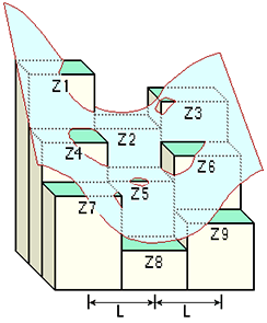
For each cell, a fourth-order polynomial of the form:
Z = Ax²y² + Bx²y + Cxy² + Dx² + Ey² + Fxy + Gx + Hy + IThe relationships between the coefficients and the nine values of elevation for every cell numbered as shown on the diagram are as follows:

 A = [(Z1 + Z3 + Z7 + Z9) / 4  - (Z2 + Z4 + Z6 + Z8) / 2 + Z5] / L4 B = [(Z1 + Z3 - Z7 - Z9) /4 - (Z2 - Z8) /2] / L3 C = [(-Z1 + Z3 - Z7 + Z9) /4 + (Z4 - Z6)] /2] / L3 D = [(Z4 + Z6) /2 - Z5] / L2 E = [(Z2 + Z8) /2 - Z5] / L2 F = (-Z1 + Z3 + Z7 - Z9) / 4L2 G = (-Z4 + Z6) / 2L
 H = (Z2 - Z8) / 2L
 I = Z5
The output of the Curvature tool is the second derivative of the surface—for example, the slope of the slope—such that:
Curvature = -2(D + E) * 100From an applied viewpoint, the output of the tool can be used to describe the physical characteristics of a drainage basin in an effort to understand erosion and runoff processes. The slope affects the overall rate of movement downslope. Aspect defines the direction of flow. The profile curvature affects the acceleration and deceleration of flow and, therefore, influences erosion and deposition. The planform curvature influences convergence and divergence of flow.
Displaying contours over a raster may help with understanding and interpreting the data resulting from the execution of the Curvature tool. An example of the process follows:
Interpreting results from Curvature
Displaying contours over a raster may help with understanding and interpreting the data resulting from the execution of the tool. An example of the process follows.
- Create a curvature raster:
Input raster : elev_ras
Output curvature raster : curv_ras
Z factor : 1
Output profile curve raster : profile_ras
Output plan curve raster : plan_ras
- Create contours of the surface raster:
Input raster : elev_ras
Output polyline features : cont_lines
Contour interval : 100
Base contour : ""
Z factor : 1
- Create a slope raster:
Input raster : elev_ras
Output raster : slope_ras
Output measurement : DEGREE
Z factor : 1
- Then create contours of the slope:
Input raster : slope_ras
Output polyline features : cont_slope
Contour interval : 5
Base contour : ""
Z factor : 1
Add the curvature raster as a layer in ArcMap. Overlay the two contour feature datasets just created and apply different color symbology for each.
References
Moore, I. D., R. B. Grayson, and A. R. Landson. 1991. Digital Terrain Modelling: A Review of Hydrological, Geomorphological, and Biological Applications. Hydrological Processes 5: 3–30.
Zeverbergen, L. W., and C. R. Thorne. 1987. Quantitative Analysis of Land Surface Topography. Earth Surface Processes and Landforms 12: 47–56.