The Similarity Search tool identifies which Candidate Features are most similar (or most dissimilar) to one or more Input Features To Match. Similarity is based on a specified list of numeric attributes (Attributes Of Interest). If more than one Input Features To Match is specified, similarity is based on averages for each of the Attributes Of Interest. The output feature class (Output Features) will contain the Input Features To Match along with all of the matching Candidate Features that were found, ordered by similarity (as specified by the Most Or Least Similar parameter). The number of matches returned is based on the value for the Number Of Results parameter.
Potential applications
- You might use the Similarity Search tool to find other cities that are just like your own city in terms of population, education, and proximity to specific recreational opportunities.
- Local officials may want to promote their city to potential businesses in order to increase tax-based revenues. The Similarity Search tool will help them identify other cities like theirs so they can compare themselves with regard to attractor attributes (such as low crime and high growth). These officials might also be interested in finding locations just like them, but either larger or smaller (cosine similarity). Finding they are similar to smaller or larger places that have been attractive to the businesses they want to entice will allow them to point out the similarities while either emphasizing the advantages of being smaller (less congestion, small town flavor) or of being larger (more potential customers). These officials might also be interested in cities that are least like them. If any of the least similar places represent competition for the businesses they want to attract, this analysis will provide information they need to present a comparison.
- A human resources manager may want to be able to justify company salary ranges. Once she identifies cities that are similar in terms of size, cost of living, and amenities, she can examine the salary ranges for those cities to see if they are in line.
- A crime analyst wants to search the database to see if a crime is part of a larger pattern or trend.
- An after-school fitness program was extremely successful in Town A. Promoters want to find other towns with similar characteristics as candidates for program expansion.
- A law enforcement agency has uncovered areas where drugs are being grown or manufactured. Identifying locations with similar characteristics may help them target future searches.
- A large retailer has several successful stores and a few underperformers. Finding locations with similar demographic and contextual characteristics (accessibility, visibility, complementary businesses, and so on) will help identify the best locations for a new store.
Matching methods
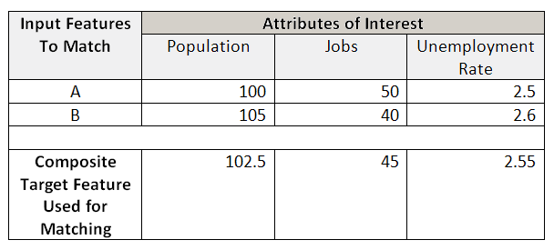
Matching may be based on attribute values, ranked attribute values, or attribute profiles (cosine similarity). The algorithm employed for each of these methods is described below. For all methods if there is more than one Input Features To Match, the attributes for all features are averaged to create a composite target feature to use for the matching process: 
Attribute values
When you select ATTRIBUTE_VALUES for the Match Method parameter, the tool first standardizes all of the Attributes of Interest. For each candidate it then subtracts the standardized values from those of the target, squares the differences, and adds the squared differences together. This sum becomes the similarity index for that candidate. Once all candidates have been processed, candidates are ranked from smallest index (most similar) to largest index (least similar).
Ranked attribute values
When you select RANKED_ATTRIBUTE_VALUES for the Match Method parameter, the tool will begin by ranking each of the Attributes of Interest both for the target feature and all of the candidates. For each candidate it then sums the squared difference for each attribute in relation to the target feature. If the population value for the target is the 10th largest among all candidates, and the population for the candidate being considered is 15th largest, the sum of the squared rank population difference for this candidate would be 10 - 15 = -5 and -5**2 is 25. The sum of squared rank differences for all of the Attributes of Interest becomes the similarity index for this candidate. Once all candidates have been processed, candidates are ranked from smallest index (most similar) to largest index (least similar).
Attribute profiles
When you select ATTRIBUTE_PROFILES for the Match Method parameter, the tool first standardizes all of the Attributes of Interest (a minimum of two Attributes of Interest is required for this method). It then uses cosine similarity mathematics to compare the vector of standardized attributes for each candidate to the vector of standardized attributes for the target feature being matched. The cosine similarity of two vectors, A and B, is computed as:

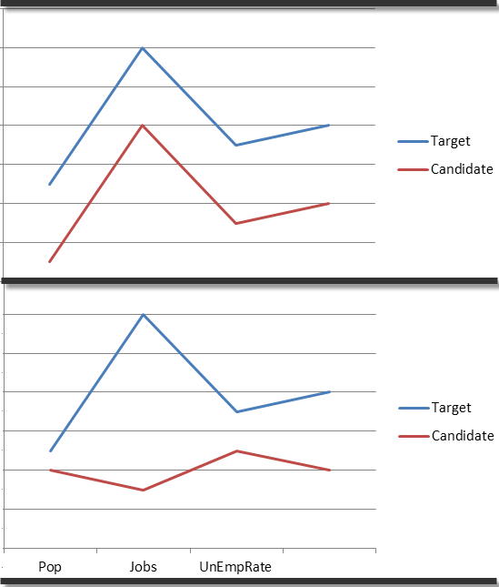
Cosine similarity is not concerned with the matching of attribute magnitudes but rather this method focuses on the relationships among the attributes. If you created a profile (line graph) of the standardized attributes in the vectors being compared (the target and one of the candidates), you might see very similar profiles or very different profiles:

The cosine similarity index ranges from 1.0 (perfect similarity) to -1.0 (perfect dissimilarity) and is reported in the SIMINDEX (Cosine Similarity) field. You would use this similarity method to find places that have the same characteristics but perhaps at a larger or smaller scale.
Best practices
Mapping similarity patterns
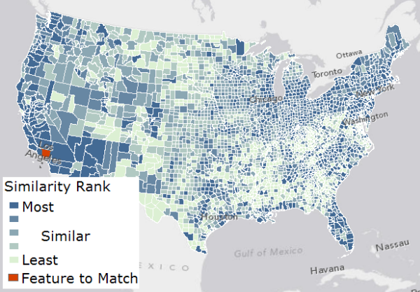
If you set the Number of Results parameter to zero, the tool will rank all of the candidate features. The output for this analysis will show you the spatial pattern of similarity. Notice that when you rank all candidates you get information about similarity and about dissimilarity.

Including spatial variables
Suppose you know the locations (polygon areas) where a particular endangered species is doing well and you want to find other locations where it might also thrive. You would be looking for locations similar to the successful ones, but might also need locations large enough and compact enough to ensure species success. For this analysis you could compute a compactness metric for each polygon area (common compactness measurements are based on the area of a polygon in relation to the area of a circle with the same perimeter). You could then include your compactness measurement and an attribute reflecting polygon size (Shape_Area) in the Fields To Append To Output parameter when you run the Similarity Search tool. Sorting the top ten solution matches in terms of both compactness and area will help you identify the most appropriate locations for species reintroduction.
Perhaps you are a retailer interested in expanding. If you have existing stores that have been successful you can use attributes reflecting the key characteristics of success to help you find candidate locations for expansion. Suppose that the products you sell will be most attractive to college students and that you want to avoid locations near your current stores or near competitors. Before running the Similarity Search tool you would use the Near tool to create your spatial variables: distance to colleges or places with high densities of college students, distance to existing stores, and distance to competitors. You could then include these spatial variables in the Fields To Append To Output parameter when you run the Similarity Search tool.