Ordinary Least Squares (OLS)

Summary

Performs global Ordinary Least Squares (OLS) linear regression to generate predictions or to model a dependent variable in terms of its relationships to a set of explanatory variables.

You can access the results of this tool (including the optional report file) from the Results window. If you disable background processing, results will also be written to the Progress dialog box.

Learn more about how Ordinary Least Squares regression works

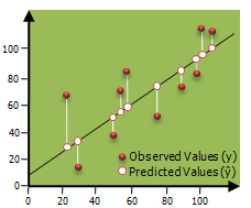
Illustration

Ordinary Least Squares Regression: predicted values in relation to observed values

Usage

• The primary output for this tool is a report file which is written to the Results window. Right-clicking on the Messages entry in the Results window and selecting View will display the Exploratory Regression summary report in a Message dialog box.

  Note:

  If this tool is part of a custom model tool, the optional tables will only appear in the Results window if they are set as model parameters prior to running the tool.

• The OLS tool also produces an output feature class and optional tables with coefficient information and diagnostics. All of these are accessible from the Results window. The output feature class is automatically added to the table of contents, with a hot/cold rendering scheme applied to model residuals. A full explanation of each output is provided in Interpreting OLS results.

• Results from OLS regression are only trustworthy if your data and regression model satisfy all of the assumptions inherently required by this method. Consult the table Common Regression Problems, Consequences, and Solutions in Regression Analysis Basics to ensure your model is properly specified.

• Dependent and Explanatory variables should be numeric fields containing a variety of values. OLS cannot solve when variables have all the same value (all the values for a field are 9.0, for example). Linear regression methods, like OLS, are not appropriate for predicting binary outcomes (for example, all of the values for the dependent variable are either 1 or 0).

• The Unique ID field links model predictions to each feature. Consequently, the Unique ID values must be unique for every feature, and typically should be a permanent field that remains with the feature class. If you don't have a Unique ID field, you can easily create one by adding a new integer field to your feature class table and calculating the field values to be equal to the FID/OID field. You cannot use the FID/OID field directly for the Unique ID parameter.

• Whenever there is statistically significant spatial autocorrelation of the regression residuals the OLS model will be considered misspecified and, consequently, results from OLS regression are unreliable. Be sure to run the Spatial Autocorrelation tool on your regression residuals to assess this potential problem. Statistically significant spatial autocorrelation of regression residuals almost always indicates one or more key explanatory variables are missing from the model.

• You should visually inspect the over- and underpredictions evident in your regression residuals to see if they provide clues about potential missing variables from your regression model. It sometimes helps to run Hot Spot Analysis on the residuals to help you visualize spatial clustering of the over- and underpredictions.

• When misspecification is the result of trying to model nonstationary variables using a global model (OLS is a global model), then Geographically Weighted Regression may be used to improve predictions and to better understand the nonstationarity (regional variation) inherent in your explanatory variables.

• When the result of a computation is infinity or undefined, the output for nonshapefiles will be Null; for shapefiles the output will be -DBL_MAX (-1.7976931348623158e+308, for example).

• Model summary diagnostics are written to the OLS summary report and the optional diagnostic output table. Both include diagnostics for the corrected Akaike Information Criterion (AICc), Coefficient of Determination, Joint F statistic, Wald statistic, Koenker's Breusch-Pagan statistic, and the Jarque-Bera statistic. The diagnostic table also includes uncorrected AIC and Sigma-squared values.

• The optional coefficient and/or diagnostic output tables, if they already exist, will be overwritten when the Geoprocessing Option to overwrite the outputs of geoprocessing operations is checked on.

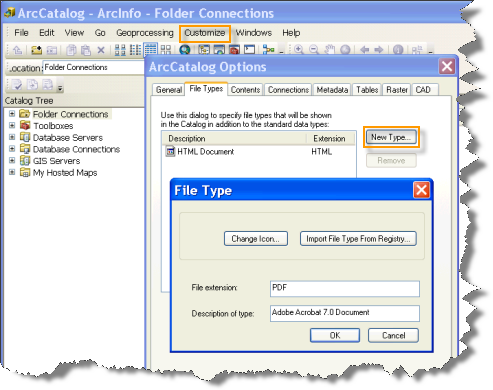
• This tool will optionally create a PDF report summarizing results. PDF files do not automatically appear in the Catalog window. If you want PDF files to be displayed in Catalog, open the ArcCatalog application, select the Customize menu option, click ArcCatalog Options, and select the File Types tab. Click on the New Type button and specify PDF, as shown below, for File Extension.

  

• On machines configured with the ArcGIS language packages for Arabic and other right-to-left languages, you might notice missing text or formatting problems in the PDF Output Report File. These problems are addressed in this article.

• Map layers can be used to define the Input Feature Class. When using a layer with a selection, only the selected features are included in the analysis.

Caution:

When using shapefiles, keep in mind that they cannot store null values. Tools or other procedures that create shapefiles from nonshapefile inputs may store or interpret null values as zero. In some cases, nulls are stored as very large negative values in shapefiles. This can lead to unexpected results. See Geoprocessing considerations for shapefile output for more information.

Syntax

OrdinaryLeastSquares(Input_Feature_Class, Unique_ID_Field, Output_Feature_Class, Dependent_Variable, Explanatory_Variables, {Coefficient_Output_Table}, {Diagnostic_Output_Table}, {Output_Report_File})

Parameter	Explanation	Data Type
Input_Feature_Class	The feature class containing the dependent and independent variables for analysis.	Feature Layer
Unique_ID_Field	An integer field containing a different value for every feature in the Input Feature Class.	Field
Output_Feature_Class	The output feature class to receive dependent variable estimates and residuals.	Feature Class
Dependent_Variable	The numeric field containing values for what you are trying to model.	Field
Explanatory_Variables [Explanatory_Variables,...]	A list of fields representing explanatory variables in your regression model.	Field
Coefficient_Output_Table (Optional)	The full path to an optional table that will receive model coefficients, standardized coefficients, standard errors, and probabilities for each explanatory variable.	Table
Diagnostic_Output_Table (Optional)	The full path to an optional table that will receive model summary diagnostics.	Table
Output_Report_File (Optional)	The path to the optional PDF file you want the tool to create. This report file includes model diagnostics, graphs, and notes to help you interpret the OLS results.	File

Code sample

OrdinaryLeastSquares example 1 (Python window)

The following Python window script demonstrates how to use the OrdinaryLeastSquares tool.

import arcpy
arcpy.env.workspace = r"c:\data"
arcpy.OrdinaryLeastSquares_stats("USCounties.shp", "MYID","olsResults.shp", 
                                 "GROWTH","LOGPCR69;SOUTH;LPCR_SOUTH;PopDen69",
                                 "olsCoefTab.dbf","olsDiagTab.dbf")

OrdinaryLeastSquares example 2 (stand-alone Python script)

The following stand-alone Python script demonstrates how to use the OrdinaryLeastSquares tool.

# Analyze the growth of regional per capita incomes in US
# Counties from 1969 -- 2002 using Ordinary Least Squares Regression

# Import system modules
import arcpy

# Set property to overwrite existing outputs
arcpy.env.overwriteOutput = True

# Local variables...
workspace = r"C:\Data"

try:
    # Set the current workspace (to avoid having to specify the full path to the feature classes each time)
    arcpy.env.workspace = workspace

    # Growth as a function of {log of starting income, dummy for South
    # counties, interaction term for South counties, population density}
    # Process: Ordinary Least Squares... 
    ols = arcpy.OrdinaryLeastSquares_stats("USCounties.shp", "MYID", 
                        "olsResults.shp", "GROWTH",
                        "LOGPCR69;SOUTH;LPCR_SOUTH;PopDen69",
                        "olsCoefTab.dbf",
                        "olsDiagTab.dbf")

    # Create Spatial Weights Matrix (Can be based off input or output FC)
    # Process: Generate Spatial Weights Matrix... 
    swm = arcpy.GenerateSpatialWeightsMatrix_stats("USCounties.shp", "MYID",
                        "euclidean6Neighs.swm",
                        "K_NEAREST_NEIGHBORS",
                        "#", "#", "#", 6) 
                        

    # Calculate Moran's Index of Spatial Autocorrelation for 
    # OLS Residuals using a SWM File.  
    # Process: Spatial Autocorrelation (Morans I)...      
    moransI = arcpy.SpatialAutocorrelation_stats("olsResults.shp", "Residual",
                        "NO_REPORT", "GET_SPATIAL_WEIGHTS_FROM_FILE", 
                        "EUCLIDEAN_DISTANCE", "NONE", "#", 
                        "euclidean6Neighs.swm")

except:
    # If an error occurred when running the tool, print out the error message.
    print(arcpy.GetMessages())

Environments

• Output Coordinate System
• Geographic Transformations
• Current Workspace
• Scratch Workspace
• Qualified Field Names
• Output has M values
• M Resolution
• M Tolerance
• Output has Z values
• Default Output Z Value
• Z Resolution
• Z Tolerance
• XY Resolution
• XY Tolerance

Licensing information

• Basic: Yes
• Standard: Yes
• Advanced: Yes