In this topic
About geoprocessing
Geoprocessing involves delivering information through analysis of existing data as well as automating batch procedures in a GIS. The following examples highlight using geoprocessing tools for data management and for building GIS solutions for complex tasks.
Data management
This workflow uses two geoprocessing tools, Project and Clip. This is an example of an infinite number of workflows you can automate with geoprocessing.
Suppose you've received 20 coverages and shapefiles from a colleague. The coverages and shapefiles are in different map projections and contain features that are outside your study area. Your task is to change the map projection of each of the 20 datasets, remove the extraneous features (clip the datasets), and put them all into a file geodatabase.
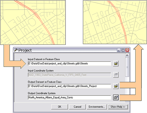
The easiest way to accomplish this task is to use geoprocessing. First, use the geoprocessing Project tool, which applies a new projection to an input feature class to create an output feature class. The following illustration shows the Project tool dialog box with its input features shown in the upper left and the projected features in the upper right. The projected coordinate system is Albers Equal Area Conic.

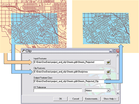
Use the geoprocessing Clip tool to clip the data that falls outside your study area. The Clip tool takes two inputs—a feature class of any type (point, polyline, or polygon) and a polygon feature class (the clip feature class)—and creates a new feature class of those features that fall inside the clip polygons. The Clip tool dialog box is shown in the following illustration:

You can also create a geoprocessing model that chains together the Project and Clip tools, feeding the output of Project into the input of Clip, and use the model in batch mode. The model you create becomes a new tool in your geoprocessing environment. This model is shown in the following diagram:

Geographic analysis
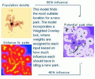
This workflow is a more complex use of geoprocessing that performs a simplified site selection for parks and produces a dataset of potential park sites that can be further evaluated. The site selection logic is to find areas that are close to densely populated areas but are not close to existing parks, the premise being that you want parks close to people, but you don't want parks clustered tightly together. It's also more important to have parks close to populated areas than it is to place a new park further away from existing parks. This is simple logic to identify potential sites for further evaluation (such as compatible land use, site availability, and site qualities).
In the following illustration, the potential park sites map shows more suitable locations in dark purple, while less suitable areas are shown in lighter shades. Gray areas mark the locations of existing parks. The illustration also shows that population density is a more influential factor; that is, it has a higher influence (60) in site selection than does distance to parks (40). (These weights are entirely arbitrary.)

- Process 1 calculates the population density from an input point feature class containing population centroids, and outputs a raster dataset containing population density for every cell.
- Process 2 calculates the distance to parks from a raster of existing parks and outputs a raster dataset with distance to existing parks as the value for each cell.
- Process 3 reclassifies the population density output.
- Process 4 reclassifies the distance to parks output.
Both reclassification processes (3 and 4) transform the raw cell values into values between zero and 100. The reclassified values score usefulness, where zero is least useful and 100 is most useful. For example, a cell that is close to an existing park scores lower than a cell further away, and a cell that has high population density scores higher than a cell with low population density. - Process 5 takes the output data from the two reclassifications and inputs the data to the Weighted Overlay process, where the weights (60 and 40) are applied (in weighted overlay, the sum of the weights should add up to 100). The output raster contains a suitability score, as shown in the model. The most suitable areas have a higher value in the output cell and are shown in dark purple.

The weighted overlay approach to screening for potential sites has been in use since before the advent of computers and GIS. Geoprocessing makes weighted overlay easy and accessible. For example, you can change the weights from 60 and 40 to other values and execute the model again to help determine the sensitivity to the weights. You can change the reclassification values as well.
You can also create GIS workflows by building custom geoprocessing tools in Java that are specific to your requirements. These custom tools can be used along with other ArcGIS tools in ModelBuilder as well. For more information on how to create custom tools, see How to build custom geoprocessing tools.
See Also:
How to build custom geoprocessing toolsCreating a custom function tool class
Creating a custom function factory
| Development licensing | Deployment licensing |
|---|---|
| Engine Developer Kit | Engine |
| Server | Server |
| ArcGIS for Desktop Basic | ArcGIS for Desktop Basic |
| ArcGIS for Desktop Standard | ArcGIS for Desktop Standard |
| ArcGIS for Desktop Advanced | ArcGIS for Desktop Advanced |