Disponible con una licencia de Geostatistical Analyst.
Most of the interpolation methods provided by ArcGIS Geostatistical Analyst do not require the data to be normally distributed, although in this case the prediction map may not be optimal. That is, data transformations that change the shape (distribution) of the data are not required as part of the interpolation model. However, certain kriging methods require the data to be approximately normally distributed (close to a bell-shaped curve). In particular, quantile and probability maps created using ordinary, simple, or universal kriging assume that the data comes from a multivariate normal distribution. In addition, simple kriging models, which are used as a basis for geostatistical simulation (that is, models used as input to the Gaussian Geostatistical Simulation tool—refer to Geostatistical simulation concepts and How Gaussian geostatistical simulations work), should use data that is normally distributed or include a normal score transformation as part of the model to ensure this.
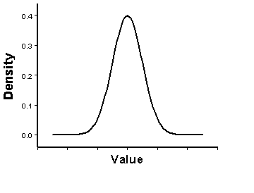
Normally distributed data has a probability density function that looks like the one shown in the following diagram:

The Histogram and Normal QQ plot are designed to help you explore the distribution of your data, and they include different data transformations (Box–Cox, logarithmic, and arcsine) so that you can assess the effects they have on the data. To learn more about the transformations that are available in these tools, see Box-Cox, Arcsine, and Log transformations.
All kriging methods rely on the assumption of stationarity. This assumption requires, in part, that all data values come from distributions that have the same variability. Data transformations can also be used to satisfy this assumption of equal variability. For more information on stationarity, see Random processes with dependence.
¿Algún comentario sobre este tema?