Disponible con una licencia de Geostatistical Analyst.
The semivariogram depicts the spatial autocorrelation of the measured sample points. Once each pair of locations is plotted (Binning the empirical semivariogram), a model is fit through them (Fitting a model to the empirical semivariogram). There are certain characteristics that are commonly used to describe these models.
The range and sill
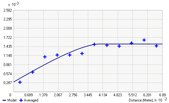
When you look at the model of a semivariogram, you'll notice that at a certain distance, the model levels out. The distance where the model first flattens out is known as the range. Sample locations separated by distances closer than the range are spatially autocorrelated, whereas locations farther apart than the range are not.
The value that the semivariogram model attains at the range (the value on the y-axis) is called the sill. The partial sill is the sill minus the nugget.

The nugget
Theoretically, at zero separation distance (lag = 0), the semivariogram value is 0. However, at an infinitesimally small separation distance, the semivariogram often exhibits a nugget effect, which is some value greater than 0. For example, if the semivariogram model intercepts the y-axis at 2, then the nugget is 2.
The nugget effect can be attributed to measurement errors or spatial sources of variation at distances smaller than the sampling interval or both. Measurement error occurs because of the error inherent in measuring devices. Natural phenomena can vary spatially over a range of scales. Variation at microscales smaller than the sampling distances will appear as part of the nugget effect. Before collecting data, it is important to gain some understanding of the scales of spatial variation.