Disponible con una licencia de Geostatistical Analyst.
Cokriging uses information on several variable types. The main variable of interest is Z1, and both autocorrelation for Z1 and cross-correlations between Z1 and all other variable types are used to make better predictions. It is appealing to use information from other variables to help make predictions, but it comes at a price. Cokriging requires much more estimation, including estimating the autocorrelation for each variable as well as all cross-correlations. Theoretically, you can do no worse than kriging because if there is no cross-correlation, you can fall back on autocorrelation for Z1. However, each time you estimate unknown autocorrelation parameters, you introduce more variability, so the gains in precision of the predictions may not be worth the extra effort.
Ordinary cokriging assumes the following two models:
Z1(s) = µ1 + ε1(s)Z2(s) = µ2 + ε2(s),where µ1 and µ2 are unknown constants.
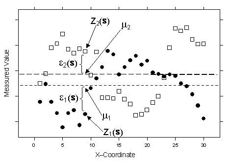
Notice that now you have two types of random errors, ε1(s) and ε2(s), so there is autocorrelation for each of them and cross-correlation between them. Ordinary cokriging attempts to predict Z1(s0), just like ordinary kriging, but it uses information in the covariate Z2(s) in an attempt to do a better job. For example, the following figure has the same data that was used for ordinary kriging, only here a second variable is added.
Notice that Z1 and Z2 both appear autocorrelated. Also notice that when Z1 is below its mean µ1, then Z2 is often above its mean µ2, and vice versa. Thus, Z1 and Z2 appear to have negative cross-correlation. In this example, each location s had both Z1(s) and Z2(s); however, this is not necessary, and each variable type can have its own unique set of locations. The main variable of interest is Z1, and both autocorrelation and cross-correlation are used to make better predictions.

The other cokriging methods—universal, simple, indicator, probability, and disjunctive—are generalizations of the foregoing methods to the case where you have multiple datasets. For example, indicator cokriging can be implemented by using several thresholds for your data and then using the binary data on each threshold to predict the threshold of primary interest. In this way, it is similar to probability kriging but can be less sensitive to outliers and other erratic data.
Semivariograms or covariances (the mathematical forms used to express autocorrelation), cross-covariance (the mathematical form used to express cross-correlation), transformations, trend removal, and measurement error can be used when performing ordinary, simple, or universal cokriging.