Disponible avec une licence Geostatistical Analyst.
Some methods in Geostatistical Analyst require that the data be normally distributed. When the data is skewed (the distribution is lopsided), you might want to transform the data to make it normal. The Histogram and Normal QQ Plot allow you to explore the effects of different transformations on the distribution of the dataset. If the interpolation model you build uses one of the kriging methods, and you choose to transform the data as one of the steps, the predictions will be transformed back to the original scale in the interpolated surface.
Geostatistical Analyst allows the use of several transformations including Box-Cox (also known as power transformations), arcsine, and logarithmic. Suppose you observe data Z(s), and apply some transformation Y(s) = t(Z(s)). Usually, you want to find the transformation so that Y(s) is normally distributed. What often happens is that the transformation also yields data that has constant variance through the study area.
Learn more about transformations and trends
Learn more about Box–Cox, arcsine, and log transformations
Box-Cox transformation
The Box-Cox transformation is
Y(s) = (Z(s)λ - 1)/λ,for λ≠ 0.
For example, suppose that your data is composed of counts of some phenomenon. For these types of data, the variance is often related to the mean. That is, if you have small counts in part of your study area, the variability in that local region will be smaller than the variability in another region where the counts are larger. In this case, the square-root transformation may help to make the variances more constant throughout the study area and often makes the data appear normally distributed as well. The square-root transformation is a special case of the Box-Cox transformation when λ = ½.
Log transformation
The log transformation is actually a special case of the Box-Cox transformation when λ = 0; the transformation is as follows:
Y(s) = ln(Z(s)),for Z(s) > 0, and ln is the natural logarithm.
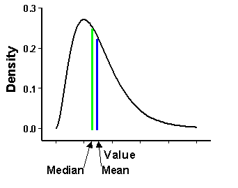
The log transformation is often used where the data has a positively skewed distribution (shown below) and there are a few very large values. If these large values are located in your study area, the log transformation will help make the variances more constant and normalize your data. Concerning terminology, when a log transformation is implemented with kriging, the prediction method is known as lognormal kriging, whereas for all other values of λ, the associated kriging method is known as trans-Gaussian kriging.

Arcsine transformation
The arcsine transformation is shown below:
Y(s) = sin-1(Z(s)),for Z(s) between 0 and 1.
The arcsine transformation can be used for data that represents proportions or percentages. Often, when the data is proportions, the variance is smallest near 0 and 1 and largest near 0.5. The arcsine transformation will help make the variances more constant throughout your study area and often makes the data appear normally distributed as well.