Disponible avec une licence Geostatistical Analyst.
By exploring your data, you'll gain a better understanding of the spatial autocorrelation among the measured values. This understanding can be used to make better decisions when choosing models for spatial prediction.
Spatial autocorrelation
You can explore the spatial autocorrelation in your data by examining the different pairs of sample locations. By measuring the distance between two locations and plotting the difference squared between the values at the locations, a semivariogram cloud is created. On the x-axis is the distance between the locations, and on the y-axis is the difference of their values squared. Each dot in the semivariogram represents a pair of locations, not the individual locations on the map.
If spatial correlation exists, pairs of points that are close together (on the far left of the x-axis) should have less difference (be low on the y-axis). As points become farther away from each other (moving right on the x-axis), in general, the difference squared should be greater (moving up on the y-axis). Often there is a certain distance beyond which the squared difference levels out. Pairs of locations beyond this distance are considered to be uncorrelated.
A fundamental assumption for geostatistical methods is that any two locations that have a similar distance and direction from each other should have a similar difference squared. This relationship is called stationarity.
Learn more about geostatistical methods that are based on statistical models
Spatial autocorrelation may depend only on the distance between two locations, which is called isotropy. However, it is possible that the same autocorrelation value may occur at different distances when considering different directions. Another way to think of this is that things are more alike for longer distances in some directions than in other directions. This directional influence is seen in semivariograms and covariances and is called anisotropy.
It is important to look for anisotropy so that if you detect directional differences in the autocorrelation, you can account for them in the semivariogram or covariance models. This in turn has an effect on the geostatistical prediction.
Exploring spatial structure through the Semivariogram/Covariance Cloud tool
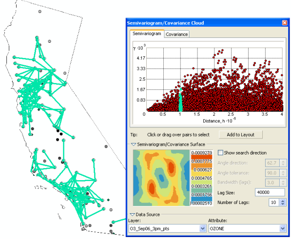
The Semivariogram/Covariance Cloud tool can be used to investigate autocorrelation in your dataset. Consider the ozone dataset. Notice in the figure below that you can select all pairs of locations that are a certain distance apart by brushing all points at that distance in the semivariogram cloud.

Looking for directional influences with the Semivariogram/Covariance Cloud tool
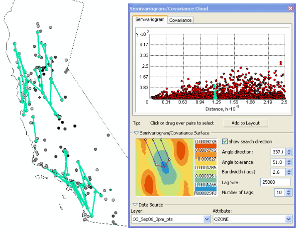
In the previous example, you used the Semivariogram/Covariance Cloud tool to look at the general autocorrelation of the data. However, looking at the semivariogram surface, it appears that there might be directional differences in the semivariogram values. When you click Show search direction and set the angles and bandwidths as in the following figure, you can see that the locations linked together have very similar values because the semivariogram values are relatively low.

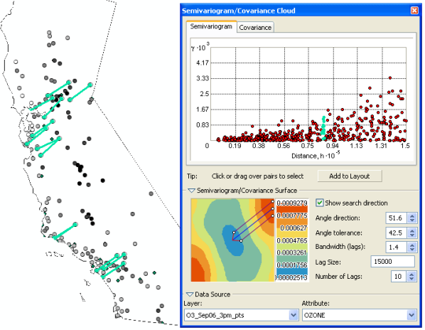
If you change the direction of the links as in the following figure, you can see that some linked locations have values that are quite different, which result in the higher semivariogram values. This indicates that locations separated by a distance of about 125,000 meters in the northeast direction are, on average, more different than locations in the northwest direction. Recall that when variation changes more rapidly in one direction than another, it is termed anisotropy. When interpolating a surface using the Geostatistical Analyst wizard, you can use semivariogram models that account for anisotropy.
