Disponible avec une licence Geostatistical Analyst.
Introduction
This exercise demonstrates how to use areal interpolation to take data collected at one set of polygons (the source polygons) and predict the data values for a new set of polygons (the target polygons). The data in this exercise involves obesity rates among fifth grade students in the Los Angeles area (for privacy reasons, the original data has been altered). For each school zone, every fifth grade student was sampled, and the number of obese and nonobese students was recorded (note that data is unavailable for 14 of the school zones). The goal of this exercise is to take the obesity rates collected at the school zone level and predict the obesity rates for the census block groups within the school zones. Additionally, you will predict the obesity rates in the 14 school zones that have missing data.
The graphic below shows the Los Angeles school zones symbolized by fifth grade obesity rate. Low rates are colored blue (indicating rates of under 22.5%), and high obesity rates are red (indicating rates greater than 44.7%), with green, yellow, and orange in the middle. The black polygons are the zones with missing data. On the right are the block groups in the Los Angeles area where you want to predict fifth grade obesity rates.
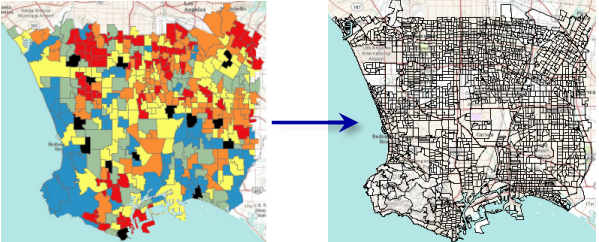
Areal interpolation is a two-step process. First, a prediction surface is created from the source polygons, then that prediction surface is averaged within the target polygons.
Create a prediction surface for obesity rates
The first step in the areal interpolation workflow is to create a prediction surface from the obesity rates collected in the school zones. Since areal interpolation requires the model to be fit interactively, the prediction surface must be created in the Geostatistical Wizard.
Open the Geostatistical Wizard
- Start ArcMap, enable the Extension ArcGIS Geostatistical Analyst, then add the Geostatistical Analyst toolbar. These steps are described at the beginning of tutorial exercise 1.
- Click the Geostatistical Analyst drop-down arrow on the Geostatistical Analyst toolbar and click Geostatistical Wizard.
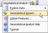
The Geostatistical Wizard dialog box appears.
Choose the method and identify the input data
- Under Geostatistical methods, click Areal Interpolation.
- Next to Type, choose Rate (binomial) since you are interested in predicting obesity rates (rather than population counts, for example).
- Next to Source Dataset, choose child_obesity to specify the polygon feature class containing the school zone obesity rates.
- Next to Count Field, choose 5th_obese.
This field contains the number of obese fifth graders.
- Next to Population Field, choose 5th_total.
This field contains the total number of fifth graders.
- Leave the defaults for Dataset 2 because you will not be using a secondary variable in this exercise.
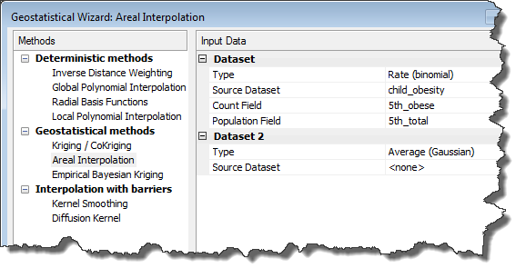
Panel 1 of the Geostatistical Wizard - Click Next to begin creating the areal interpolation model.
Adjusting the variography
You are now viewing the variography panel in the wizard. In the entire areal interpolation workflow, this step takes the most time and is the most critical for obtaining accurate predictions. The goal is to change the parameters on the right so that most empirical covariances (blue crosses) fall within the confidence intervals (red bars). If the model is specified correctly, you expect about 90 percent of the empirical covariances to fall within the confidence intervals.
You can see in the graphic below that the default model is not adequate; most of the empirical covariances do not fall in the confidence intervals. You need to do some work to make the model fit.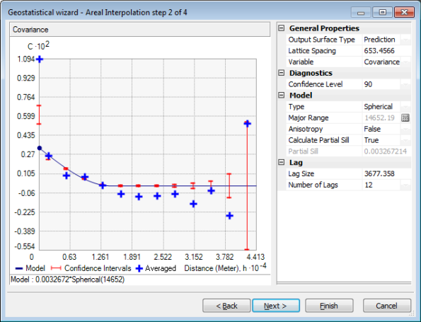
- You can see that the empirical covariances become negative at a distance of approximately 12,000 meters. This indicates that you should start by changing Lag Size to 1000 and keep Number of Lags at 12. (The product of these two parameters should approximately equal the distance where the empirical covariances first become negative.)
The covariance curve below looks better, but the model can still be improved. The large empirical covariance on the y-axis is troubling.
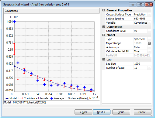
Panel 2 of the Geostatistical Wizard - To try to improve this result, under Model, change Type to K-Bessel.
This model appears to fit the data very well; most of the empirical covariances fall inside the confidence intervals, and a few fall just outside the intervals. However, before you can be confident that this is a good model, you need to check the cross-validation results.
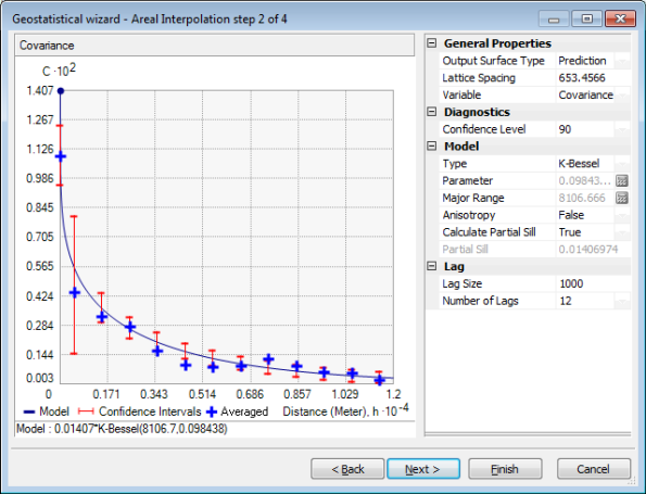
Panel 2 of the Geostatistical Wizard - Click Next to view the Searching Neighborhood panel.
Modify the search neighborhood
The Searching Neighborhood panel displays a preview surface for the fifth grade obesity rates. By clicking a point on the preview surface, you can get the predicted obesity rate at that point. For example, in the graphic below, the point (1974946, 540966.7) has a predicted value of 0.3331771. This means that the model predicts that any fifth grade student at that location has about a 33 percent chance of being obese.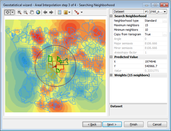
- Click Next to view the Cross Validation panel.
Examine the cross-validation
- Click the Normal QQPlot tab under the graphic on the right of the wizard's panel.
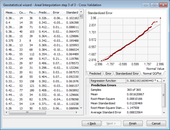
Panel 4 of the Geostatistical Wizard You can see that the Root-Mean-Square Standardized value is 1.147508. This is good because, ideally, this number should be close to 1. The normal QQ plot also reveals that the standard errors are close to being normally distributed because the points fall near the one-to-one line. This is the model that you will use to make your prediction.
- Click Finish, then click OK on the Method Report dialog box.
The prediction surface for the obesity rate is displayed in ArcMap. Depending on your analysis, this obesity rate surface may be all that you need. In that case, the workflow can end here. However, you want to predict the obesity rates of fifth grade students at the block group level, so you will continue to the second half of this areal interpolation workflow.
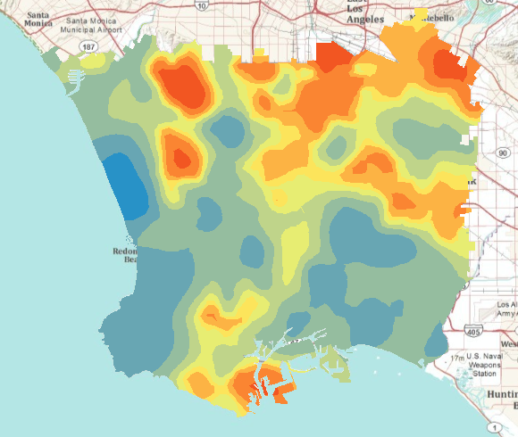
Obesity rate surface for Los Angeles fifth grade students
Predict obesity rates in census block groups
Once a proper prediction surface has been created with areal interpolation, the surface can be used to predict the fifth grade obesity rates in Los Angeles block groups using the Areal Interpolation Layer To Polygons tool.
- Right-click the 5th grade obesity layer in the ArcMap table of contents and click Predict to Polygons to open the Areal Interpolation Layer To Polygons tool dialog box.
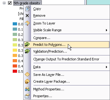
- Verify that Input areal interpolation geostatistical layer is set to 5th grade obesity.
- Click the Input polygon features drop-down arrow and click LA_blocks to specify the polygon feature class of the Los Angeles block groups.
- Click the Output polygon feature class browse button, navigate to the location where you want the output to be saved, then enter LA_blocks_obesity as the name for the output polygon feature class.
- Verify that Append all fields from input features is checked because you want to carry over all the fields from the LA_blocks feature class.
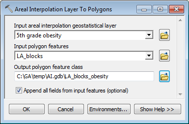
Areal Interpolation Layer To Polygons geoprocessing tool dialog box - Click OK to run the tool.
The polygon feature class containing the predictions for fifth grade obesity rates in Los Angeles block groups is added to ArcMap. The field with the predicted obesity rates is labeled Predicted. In addition, the standard errors of the prediction are stored in a field labeled StdError.
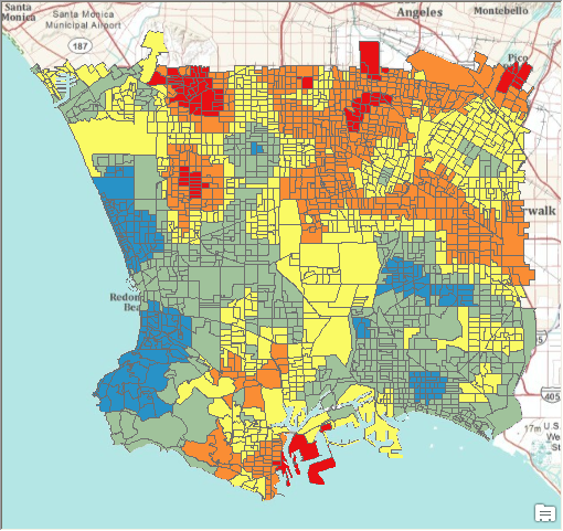
Predicted obesity rates for fifth grade students in Los Angeles block groups - You can also symbolize the block groups by the standard error of the predicted obesity rates. The standard errors are stored in the StdError field of LA_blocks_obesity. This allows you to create margins of error for the predicted obesity rates.
Low standard errors are symbolized in lighter shades of red. Larger block groups tend to have smaller standard errors because larger areas have more information associated with them, so there is less uncertainty in the predictions.
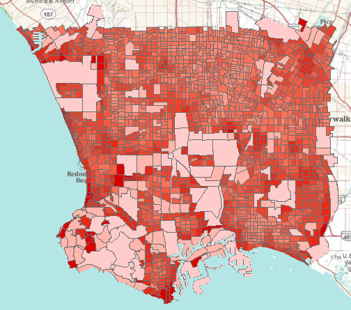
Standard errors for obesity rates in Los Angeles block groups
This completes the workflow for predicting fifth grade obesity rates in Los Angeles block groups from rates sampled in school zones.
Predict obesity rates in school zones with missing data
To predict the obesity rates in the school zones with missing data, you will use the Areal Interpolation Layer To Polygons tool again.
- Right-click the obesity rate surface layer in the ArcMap table of contents and click Predict to Polygons to open the Areal Interpolation Layer To Polygons tool dialog box.

- Verify that Input areal interpolation geostatistical layer is set to 5th grade obesity.
- Click the Input polygon features drop-down arrow and click Missing_zones to specify the polygon feature class of the school zones with missing data.
- Click the Output polygon feature class browse button, navigate to the location where you want the output to be saved, then enter Missing_zones_obesity as the name for the output polygon feature class.
- Verify that Append all fields from input features is checked because you want to carry over all the fields from the Missing_zones feature class.
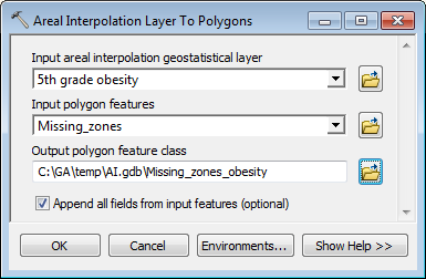
Areal Interpolation Layer To Polygons geoprocessing tool dialog box - Click OK to run the tool.
The polygon feature class containing the predictions for fifth grade obesity rates in the missing Los Angeles school zones is added to ArcMap. The field with the predicted obesity rates is labeled Predicted. In addition, the standard errors of the prediction are stored in a field labeled StdError.
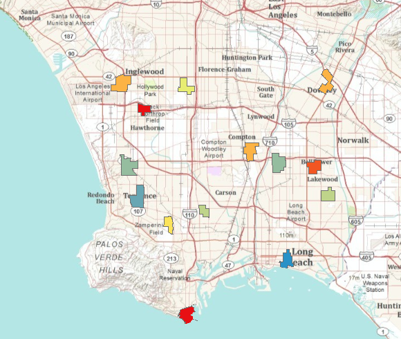
Predicted obesity rates for fifth grade students in missing school zones
You have completed the workflow for predicting fifth grade obesity rates in Los Angeles school zones where data was missing.
You can close ArcMap without saving your results.
Data reference
- Rosenshein, L. "The Local Nature of a National Epidemic: Childhood Overweight and the Accessibility of Healthy Food." M.S. dissertation, George Mason University, Department of Geography and GeoInformation Science, Fairfax, Virginia, USA, 2010.