Disponible avec une licence Geostatistical Analyst.
Probability kriging assumes the model
I(s) = I(Z(s) > ct) = µ1 + ε1(s)

Z(s) = µ2 + ε2(s),
where µ1 and µ2 are unknown constants and I(s) is a binary variable created by using a threshold indicator, I(Z(s) > ct).
Notice that now there are two types of random errors, ε1(s) and ε2(s), so there is autocorrelation for each of them and cross-correlation between them. Probability kriging strives to do the same thing as indicator kriging, but it uses cokriging in an attempt to do a better job.
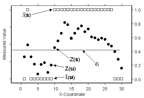
For example, in the following figure, which uses the same data as that of ordinary, universal, simple, and indicator kriging concepts, notice the datums labeled Z(u=9), which has an indicator variable of I(u) = 0, and Z(s=10), which has an indicator variable of I(s) = 1.

If you wanted to predict a value halfway between them, at x-coordinate 9.5, using indicator kriging alone would give a prediction near 0.5. However, you can see that Z(s) is just above the threshold, but Z(u) is well below the threshold. Therefore, you have some reason to believe that an indicator prediction at location 9.5 should be less than 0.5. Probability kriging tries to exploit the extra information in the original data in addition to the binary variable. However, it comes with a price. You have to do much more estimation, which includes estimating the autocorrelation for each variable as well as their cross-correlation. Each time you estimate unknown autocorrelation parameters, you introduce more uncertainty, so probability kriging may not be worth the extra effort.
Probability kriging can use either semivariograms or covariances (the mathematical forms used to express autocorrelation), cross-covariances (the mathematical forms used to express cross-correlation), and transformations, but it cannot allow for measurement error.