Geostatistical Analyst のライセンスで利用可能。
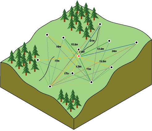
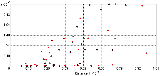
To create an empirical semivariogram, determine the squared difference between the values for all pairs of locations. When these are plotted, with half the squared difference on the y-axis and the distance that separates the locations on the x-axis, it is called the semivariogram cloud. The scene below shows the pairings of one location (the red point) with 11 other locations.

One of the main goals of variography is to explore and quantify spatial dependence, also called spatial autocorrelation. Spatial autocorrelation quantifies the assumption that things that are closer are more alike than things that are farther apart. Thus, pairs of locations that are closer (far left on the x-axis of the semivariogram cloud) would have more similar values (low on the y-axis of the semivariogram cloud). As pairs of locations become farther apart (moving to the right on the x-axis of the semivariogram cloud), they should become more dissimilar and have a higher squared difference (move up on the y-axis of the semivariogram cloud).

Due to computing limitations (computing time and memory limits), if the input dataset has more than 5000 observations, Geostatistical Analyst will randomly select 5000 observations for the structural analysis and semivariogram model fitting (this provides about 12 million pairs of points). The resulting model (surface) is usually not affected by the random sampling since all the data are used to generate the predicted values. However, if the dataset has a few very large values, they may or may not be in the subset used to generate the empirical semivariogram/covariance values, and consequently, the estimated semivariogram model may be different from a semivariogram model estimated using the entire dataset.
このトピックへのフィードバック