Geostatistical Analyst のライセンスで利用可能。
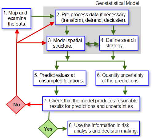
In this topic, a generalized workflow for geostatistical studies is presented, and the main steps are explained. As mentioned in What is geostatistics, geostatistics is a class of statistics used to analyze and predict the values associated with spatial or spatiotemporal phenomena. Geostatistical Analyst provides a set of tools that allow models that use spatial coordinates to be constructed. These models can be applied to a wide variety of scenarios and are typically used to generate predictions for unsampled locations, as well as measures of uncertainty for those predictions.

The first step, as in almost any data-driven study, is to closely examine the data. This typically starts by mapping the dataset, using a classification and color scheme that allow clear visualization of important characteristics that the dataset might present, for example, a strong increase in values from north to south (Trend—see Trend analysis); a mix of high and low values in no particular arrangement (possibly a sign that the data was taken at a scale that does not show spatial correlation—see Examining spatial structure and directional variation); or zones that are more densely sampled (preferential sampling) and may lead to the decision to use declustering weights in the analysis of the data—see Implementing declustering to adjust for preferential sampling. See Map the data for a more detailed discussion on mapping and classification schemes.
The second stage is to build the geostatistical model. This process can entail several steps, depending on the objectives of the study (that is, the types of information the model is supposed to provide) and the features of the dataset that have been deemed important enough to incorporate. At this stage, information collected during a rigorous exploration of the dataset and prior knowledge of the phenomenon determine how complex the model is and how good the interpolated values and measures of uncertainty will be. In the figure above, building the model can involve preprocessing the data to remove spatial trends, which are modeled separately and added back in the final step of the interpolation process (see Trend analysis); transforming the data so that it follows a Gaussian distribution more closely (required by some methods and model outputs—see Examine the distribution of the data); and declustering the dataset to compensate for preferential sampling. While a lot of information can be derived by examining the dataset, it is important to incorporate any knowledge you might have of the phenomenon. The modeler cannot rely solely on the dataset to show all the important features; those that do not appear can still be incorporated into the model by adjusting parameter values to reflect an expected outcome. It is important that the model be as realistic as possible in order for the interpolated values and associated uncertainties to be accurate representations of the real phenomenon.
In addition to preprocessing the data, it may be necessary to model the spatial structure (spatial correlation) in the dataset. Some methods, such as kriging, require this to be explicitly modeled using semivariogram or covariance functions (see Semivariograms and covariance functions, whereas other methods, such as Inverse Distance Weighting, rely on an assumed degree of spatial structure, which the modeler must provide based on prior knowledge of the phenomenon.
A final component of the model is the search strategy. This defines how many data points are used to generate a value for an unsampled location. Their spatial configuration (location with respect to one another and to the unsampled location) can also be defined. Both factors affect the interpolated value and its associated uncertainty. For many methods, a search ellipse is defined, along with the number of sectors the ellipse is split into and how many points are taken from each sector to make a prediction (see Search neighborhoods).
Once the model has been completely defined, it can be used in conjunction with the dataset to generate interpolated values for all unsampled locations within an area of interest. The output is usually a map showing values of the variable being modeled. The effect of outliers can be investigated at this stage, as they will probably change the model's parameter values and thus the interpolated map. Depending on the interpolation method, the same model can also be used to generate measures of uncertainty for the interpolated values. Not all models have this capability, so it is important to define at the start if measures of uncertainty are needed. This determines which of the models are suitable (see Classification trees).
As with all modeling endeavors, the model's output should be checked, that is, make sure that the interpolated values and associated measures of uncertainty are reasonable and match your expectations.
Once the model has been satisfactorily built, adjusted, and its output checked, the results can be used in risk analyses and decision making.