Geostatistical Analyst のライセンスで利用可能。
A global outlier is a measured sample point that has a very high or a very low value relative to all the values in a dataset. For example, if 99 out of 100 points have values between 300 and 400, but the 100th point has a value of 750, the 100th point may be a global outlier.
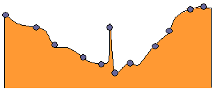
A local outlier is a measured sample point that has a value within the normal range for the entire dataset, but if you look at the surrounding points, it is unusually high or low. For example, the diagram below is a cross section of a valley in a landscape. However, there is one point in the center of the valley that has an unusually high value relative to its surroundings, but it is not unusual compared to the entire dataset.

It is important to identify outliers for two reasons: they may be real abnormalities in the phenomenon, or the value might have been measured or recorded incorrectly.
If an outlier is an actual abnormality in the phenomenon, this may be the most significant point of the study and for understanding the phenomenon. For instance, a sample on the vein of a mineral ore might be an outlier and the location that is most important to a mining company.
If outliers are caused by errors during data entry that are clearly incorrect, they should either be corrected or removed before creating a surface. Outliers can have several detrimental effects on your prediction surface because of effects on semivariogram modeling and the influence of neighboring values.
Looking for outliers through the Histogram tool
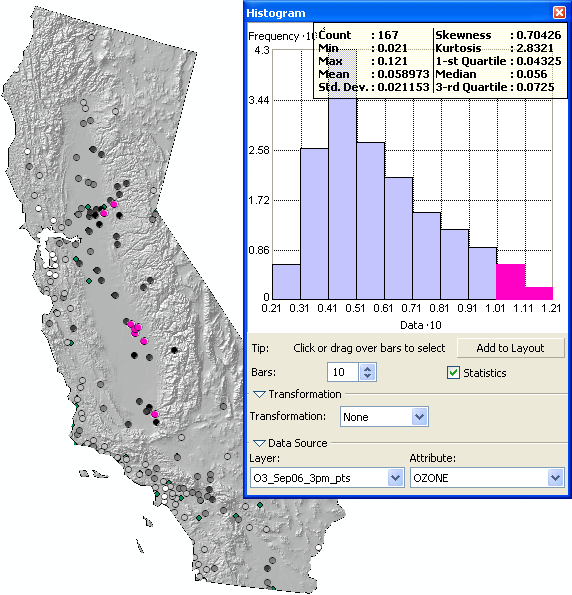
The Histogram tool enables you to select points on the tail of the distribution. The selected points are displayed in the ArcMap data view. If the extreme values are isolated locations (for instance, surrounded by very different values), they may require further investigation and be removed if necessary.

In the example above, the high ozone values are not outliers and should not be removed from the dataset.
Identifying outliers through Semivariogram/Covariance cloud
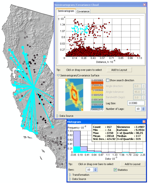
If you have a global outlier with an unusually high value in your dataset, all pairings of points with that outlier will have high values in the Semivariogram cloud, no matter what the distance is. This can be seen in the semivariogram cloud and in the histogram shown below. Notice that there are two main strata of points in the semivariogram. If you brush points in the upper strata, as demonstrated in the image, you can see in the ArcMap view that all these high values come from pairings with a single location— a global outlier. Thus, the upper stratum of points has been created by all the locations pairing with the single outlier, and the lower stratum is composed of the pairings among the rest of the locations. When you look at the histogram, you can see one high value on the right tail of the histogram, again identifying the global outlier. This value was probably entered incorrectly and should be removed or corrected.

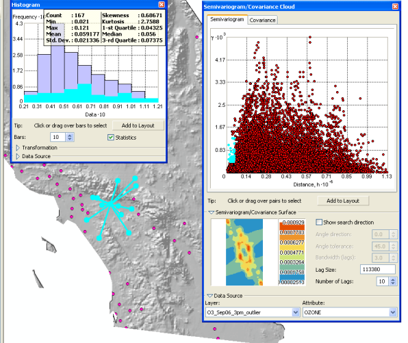
When there is a local outlier, the value will not be out of the range of the entire distribution but will be unusual relative to the surrounding values. In the local outlier histogram shown below, you can see that pairs of locations that are close together have high semivariogram values (these points are on the far left on the x-axis, indicating that they are close together, and have high values on the y-axis, indicating that the semivariogram values are high). When these points are brushed, you can see that all these points are pairings to a single location. When you look at the histogram, you can see that there is no single value that is unusual. The location in question is highlighted in the lower tail of the histogram and is paired with higher surrounding values (see the highlighted points in the histogram). This location may be a local outlier. Further investigation should be made before deciding if the value at that point is erroneous or in fact reflects a true characteristic of the phenomenon and should be included as part of the model.

Looking for outliers through Voronoi mapping
Voronoi maps based on the cluster and entropy methods can be used to identify possible outliers.
Entropy values provide a measure of dissimilarity between neighboring cells. In nature, you would expect that things closer together are more likely to be more similar than things farther apart. Therefore, local outliers may be identified by areas of high entropy.
The cluster method identifies those cells that are dissimilar to their surrounding neighbors. You would expect the value recorded in a particular cell to be similar to at least one of its neighbors. Therefore, this tool may be used to identify possible outliers.