Geostatistical Analyst のライセンスで利用可能。
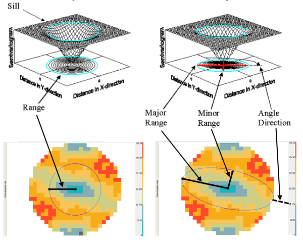
Because you are working in two-dimensional space, you might expect that the semivariogram and covariance functions change not only with distance but with direction as well. This is called anisotropy.
Learn more about semivariogram and covariance functions
Consider two points, si and sj, and the vector that separates them, which is denoted as si - sj. This vector will have a distance on the x-axis as well as the y-axis. Alternatively, you can think of the vector as having a distance and an angle in polar coordinates. Here anisotropy is described for the semivariogram; the ideas are similar for covariance functions.
The isotropic model is the same in all directions, whereas the anisotropic model reaches the sill more rapidly in some directions than others. The length of the longer axis to reach the sill is called the major range, the length of the shorter axis to reach the sill is called the minor range, and you also have the angle of rotation of the line that forms the major range. In Geostatistical Analyst, an outline of the range is given in blue, over the empirical semivariogram surface.
