Geostatistical Analyst のライセンスで利用可能。
Global polynomial interpolation fits a smooth surface that is defined by a mathematical function (a polynomial) to the input sample points. The global polynomial surface changes gradually and captures coarse-scale pattern in the data.
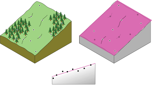
Conceptually, global polynomial interpolation is like taking a piece of paper and fitting it between the raised points (raised to the height of value). This is demonstrated in the diagram below for a set of sample points of elevation taken on a gently sloping hill (the piece of paper is magenta).

But a flat piece of paper will not accurately capture a landscape containing a valley. However, if you are allowed to bend the piece of paper once, you will get a much better fit. Adding a term to the mathematical formula produces a similar result, a bend in the plane. A flat plane (no bend in the piece of paper) is a first-order polynomial (linear). Allowing for one bend is a second-order polynomial (quadratic), two bends a third-order (cubic), and so forth; up to 10 are allowed in Geostatistical Analyst. The following image conceptually demonstrates a second-order polynomial fitted to a valley.

Rarely will the piece of paper pass through the actual measured points, thus making global polynomial interpolation an inexact interpolator. Some points will be above the piece of paper, and others will be below. However, if you add up how much higher each point is above the piece of paper and add up how much lower each point is below the piece of paper, the two sums should be similar. The surface, in magenta, is obtained by using a least-squares regression fit. The resulting surface minimizes the squared differences among the raised values and the sheet of paper.
When to use global polynomial interpolation
The result from global polynomial interpolation is a smooth surface that represents gradual trends in the surface over the area of interest.
Global polynomial interpolation is used for the following:
- Fitting a surface to the sample points when the surface varies slowly from region to region over the area of interest (for example, pollution over an industrial area).
- Examining and/or removing the effects of long-range or global trends. In such circumstances, the technique is often referred to as trend surface analysis.
Global polynomial interpolation creates a slowly varying surface using low-order polynomials that possibly describe some physical process (such as pollution and wind direction). However, it should be noted that the more complex the polynomial, the more difficult it is to ascribe physical meaning to it. Furthermore, the calculated surfaces are highly susceptible to outliers (extremely high and low values), especially at the edges.