Understanding cost distance analysis

Cost distance analysis is one of the most common applications in ArcGIS Spatial Analyst extension. Cost distance analysis can be used to solve multiple problems. Here are a few example cases:

• Constructing a road to a proposed ski area
• Supplying and reinforcing military troops
• Providing movement paths for firefighters between headquarters
• Locating a new pipeline to connect petroleum fields to a refinery
• Siting electrical lines for a new housing development
• For this case study, conserving wildlife corridors between habitat patches

Cost distance analysis simulates how a traveler moves through a landscape and should not be confused with Euclidean distance (that is, as the crow flies). Units of cost vary, and include:

• Preference
• Energy expended
• Time
• Money
• Risk

This case study identifies the steps for defining the best corridor network for bobcat to move throughout Vermont, USA. The focus of the case study is to demonstrate the various workflows to create corridor networks and least-cost paths using cost distance analysis. While creating wildlife corridors for bobcat is being used to demonstrate these workflows, the steps can be applied to most other cost distance analysis scenarios. The data and the workflow discussed in this case study are real but the actual problem and the analysis were developed for demonstration purposes. We encourage you to refine the general principles and criteria presented in the model with your specific knowledge.

Six bobcat habitat patches have been identified in Vermont using a suitability model. For a discussion of how these habitat patches were identified see Understanding the suitability modeling workflow.

Your problem statement

Continuing the scenario presented from the suitability modeling case study, you are a director in the Vermont Department of Natural Resources and you need to conserve wildlife populations that are being threatened by habitat fragmentation. New roads, housing developments, and timber harvesting have broken large tracts of contiguous forest into isolated patches that are too small for many forest-dwelling animals. To slow the rate of fragmentation, you have prioritized which lands to protect in the suitability case study identified above and now you must design a way to connect them.

Connecting isolated patches of habitat is important to maintain biodiversity and to allow individuals from different populations to create a robust metapopulation (a group of populations of the same species separated by space but with some interaction between the populations). This connectivity will allow spatially-discrete subpopulations to interact with each other to encourage genetic diversity and allows the species to recolonize a patch if the local population goes extinct.

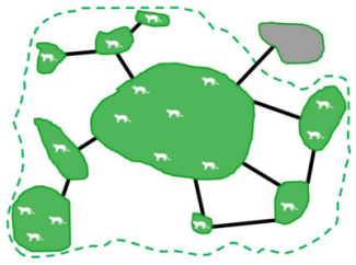
Since you cannot individually consider each wildlife species, you opt to design the conservation plan around an umbrella species. An umbrella species is a species generally high on the food chain which requires large areas of intact habitat. In this particular area, bobcat (Lynx rufus) will be your umbrella species.

By focusing your conservation efforts on protecting an umbrella species, you will indirectly protect other species with similar habitat needs. As the name implies, the bobcat acts as an umbrella for protecting other species with similar requirements.

The study site

Vermont is a small, rural state, with the Green Mountains running north-south through the center. Forest vegetation, mostly maple/hickory and spruce/fir tree types, dominates the land cover, followed by agricultural fields.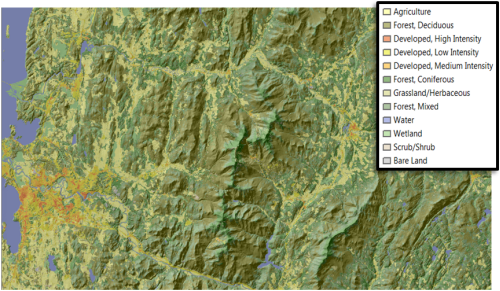

The cost distance analysis workflows

Two main workflows exist for connecting sources using cost distance analyses. The workflows can be end products in themselves or they can be synergistically combined to enhance an analysis. The two main workflows are:

1. Create a least-cost network of paths between the regions using the Cost Connectivity tool
2. Create a least-cost path between an identified source and destination using the Cost Distance and Cost Path sequence of tools

	Cost Connectivity workflow	Cost Distance/Cost Path workflow
Primary output	Network of least-cost paths connecting regions	Cost distance: identifies the least-accumulative cost for each cell to reach the cheapest source Least-cost path between a source and a destination
Secondary output	Network of least-cost paths between a region and its least-cost neighbor	Cost Allocation: for each cell, identifies the cheapest source to reach Cost back link: for each cell, identifies the direction to reach the cheapest source

In the lessons at the end of this case study, you will learn how to use both workflows in a complementary manner to create the wildlife corridor network for the bobcat to safely move between the habitat patches. You will use the Cost Connectivity workflow to produce an optimum least-cost network of paths for the bobcat and the Cost Distance/Cost Path workflow to add specific paths to the network based on a priori information that the optimum network does not capture.

Both workflows require the regions to be connected and a cost surface. The cost surface identifies the cost per map unit to move across the landscape.

This case study is divided into six sections:

1. How to create a cost surface
2. Cost distance analysis workflow one: Cost Connectivity
3. Cost distance analysis workflow two: Cost Distance/Cost Path
4. Extending workflows one and two
5. Adding complexity to cost distance analysis
6. Creating Corridors

How to create a cost surface

A cost surface represents the cost or preference of the mover to travel through each location. Cost is calculated per map unit, with each cell identifying how costly it is to move through that cell. Example cost units for cost surfaces include:

• Fire fighters: time to reach fires
• Military troops: level of security
• Bobcat: energy expended

Creating a cost surface follows similar steps to creating a suitability surface that were used to identify the six habitat patches that now need to be connected. The steps are:

1. Define the problem (which includes creating submodels).
2. Identify and derive the criteria.
3. Transform values to a common scale.
4. Weight the criteria relative to one another and combine.
5. Analyze the results.

The main difference when creating a cost surface versus a suitability surface is the cost surface is used for least-cost analysis. That is, the lower the values on the cost surface are more preferred as opposed to the higher values are better in a suitability surface. As a result, when implementing step 3, transform values to a common scale, the less costly or more preferred locations will receive lower values.

Cost surface for bobcat movement. Low cost areas are displayed as green, whereas red areas are more costly.

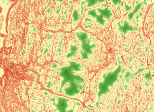
See Lesson 1: Creating a cost surface for steps on how to create a cost surface.

Cost distance analysis workflow one: Cost Connectivity

You now have the patches you want to connect derived from the suitability analysis and the cost surface identifying the cost to move through each cell. Next you want to connect the patches.

Bobcat habitat patches identified through a suitability model are displayed in blue over the cost surface.

The Cost Connectivity tool requires two inputs: the regions to be connected and a cost surface.

The Cost Connectivity tool, using a minimum spanning tree algorithm, creates the optimum network of least-cost paths connecting all the patches. Using the resulting network, each region can be reached from all other regions (possibly traveling through intermediate regions to get there).

Habitat patches connected with the least-cost network of paths derived from the minimum spanning tree algorithm using Cost Connectivity.

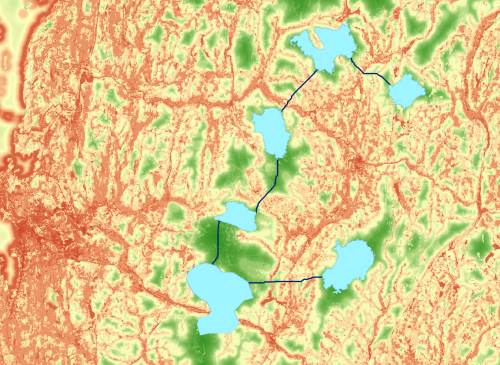
Cost Connectivity can output a second network of paths that connect each region to its neighboring cost region. From this network of paths you can remove specific paths based on a priori information or statistics associated with a path (for example, the total least accumulative cost).

For additional information, see the Cost Connectivity tool documentation and the Cost Connectivity story map.

Cost Connectivity can be used for:

• Fire fighters: creating a network of paths for traveling between multiple headquarters
• Military troops: identifying the best routes between outposts to move supplies and reinforcements
• Bobcat: ensuring breeding habitat is connected to maintain genetic diversity and allow for recolonization of habitat patches if the species goes locally extinct

Cost distance analysis workflow two: Cost Distance/Cost Path

At this point you have determined the optimum network of wildlife paths to connect the best habitat identified in the suitability modeling case study. Now you will learn how to optimally connect a specific source to a specific destination with the optimum path. You could use this capability to add specific paths to your optimum network determined by the Cost Connectivity tool described above.

In this second workflow, identifying optimum paths requires:

1. A source and cost surface
2. A destination and the cost distance and back-link rasters derived from the source and cost surface

In this example, a single region serves as a source for the input into the Cost Distance tool.

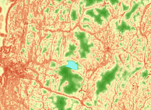
This Cost Distance/Cost Path workflow is a two step process:

1. Calculate the least-cost distance and back-link rasters from the source.
2. Create the least-cost path from the source to the destination.

Step 1: Calculate the least-cost distance and back-link rasters from the source

• From a source(s) over a cost surface, the Cost Distance tool yields an output distance raster which identifies the least accumulative cost for each cell to reach the source that is cheapest (the lowest cost) to move to. The cost-distance raster is required for step 2 of this workflow - calculating the least-cost path.

  

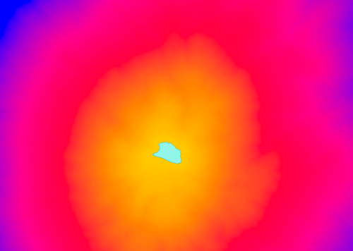
  Accumulative cost distance from the source.

• The Cost Distance tool can also produce a cost back-link raster which identifies for each cell, the cheapest direction of movement towards the source. Each cell is assigned a number identifying which neighboring cell to move into. The back-link raster is required for step 2 of this workflow - calculating the least-cost path.

  

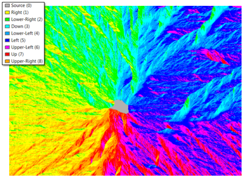
  The back-link raster from the Cost Distance tool is a directional guide for moving back to the source.

• Cost Allocation, another cost distance tool, can be used to identify, for each cell, which source is the least-costly to reach.

  

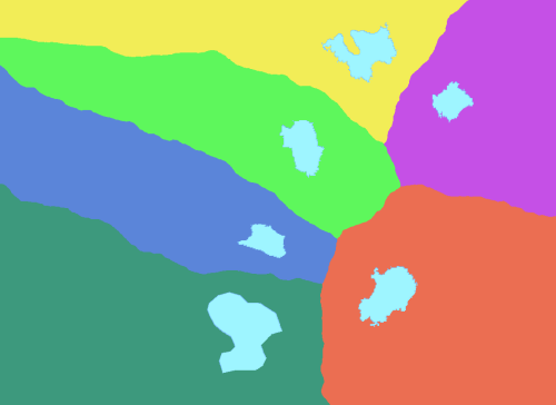
  Each location is allocated to the source that is least costly to reach.

The cost distance tools take an iterative approach to produce the cost distance raster. To learn about the formulas and algorithm used in the calculations see How the Cost distance tools work.

As a traveler moves away from the source, the overall accumulative cost increases.

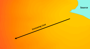
The output rasters from step one are commonly used as the input to step two of this workflow to create the least-cost path. However, the output may be used as an end product in itself. For example:

• Fire fighters: how much time it takes to reach any particular area from a headquarter, or which areas should be served by individual headquarters
• Military troops: how long it would take soldiers to trek to outposts, or which supply locations could be reached the quickest
• Bobcat: how preferred each location is based on the difficulty of the travel to reach a stream

Step 2: Create the least-cost path from the source to the destination

• Using the cost distance and cost back-link rasters from step one and a destination, the Cost Path tool calculates the least-cost path between the source and destination.

  

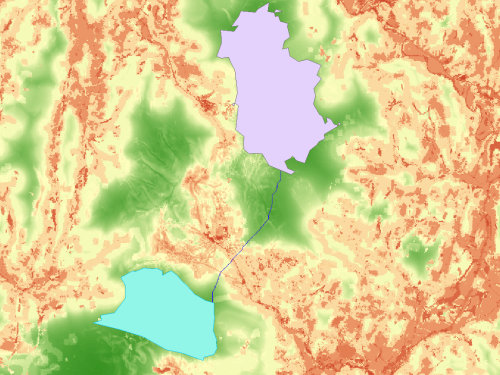
  The least-cost path (dark blue) connects the source and destination. Note how the path navigates through the cost surface.

For additional information see Cost Path tool documentation and the Exploring Cost Distance Analysis story map.

Extending workflows one and two

Workflows one and two can be end products in themselves or they can be accentuated with additional analysis.

Synergy between workflow one (Cost Connectivity) and workflow two (Cost Distance/Cost Path)

Adding least-cost paths to an optimum network or removing paths from the alternative network of paths to the cheapest neighboring regions created by Cost Connectivity in workflow one may be necessary for identifying:

• Fire fighters: the quickest access to a special park that needs protection from a forest fire
• Military troops: an alternative access route to an isolated town
• Bobcat: multiple paths to make dispersal easier for a growing population

Synergy workflow 1

1. An optimum network based on the minimum spanning tree algorithm is created using Cost Connectivity.
2. Individual paths are added for specific reasons (for example, escape/access routes) or to utilize specific capabilities (for example, source characteristics or directionality) using or within the Cost Distance/Cost Path tools.

Synergy workflow 2

1. Create all paths to neighboring cost regions with Cost Connectivity.
2. Eliminate some paths based on knowledge or the quality of the paths defined by the accompanying statistics with each path.

For additional information on how to implement these two synergistic workflows see the Getting to know Cost Connectivity story map.

Performing additional analysis in ArcGIS Network Analyst extension

Additional analysis can be done with the Cost Connectivity output within Network Analyst. The resulting network from the cost connectivity is directly compatible with Network Analyst.

Additional analysis such as route options, defining service areas, and location-allocation are common applications available through Network Analyst. Network Analyst could be used to further analyze the resulting network from cost distance analysis to identify:

• Which fire engines are closest to a fire
• Which route is the quickest for military reinforcements to respond to an attack on an outpost
• Which corridors will the animals use if a new residential development blocks an existing wildlife corridor

To explore using Network Analyst on a resulting corridor network see the FireFighting story map

Adding complexity to cost distance analysis

At this point, two main cost distance workflows have been described. The first used Cost Connectivity to create an optimum network of paths to connect a series of input regions. In the second, specific source and destinations were connected with an optimum path through a two step process using the Cost Distance/Cost Path tools.

Additional cost distance analysis functionality is available to capture more complex movement characteristics of a mover. You can add complexity to your cost analysis by:

• Controlling the characteristics of sources and the travelers from the sources
• Accounting for actual distance traveled using a surface raster
• Incorporating directionality through horizontal and vertical factors

The cost to move from one cell to another is influenced by the following:

1. The surface characteristics (the cost surface).
2. The characteristics of the mover. This could include the mode of travel, such as moving by foot or riding an ATV.
3. The characteristics of the movement when moving from one cell to another, such as whether moving uphill or downhill.

The general cost distance formula is:

Cost = Cost of travel    *  Characteristics  *  Movement characteristics
       over the surface     of the mover        on the surface

The Cost Connectivity (workflow one) and Cost Distance/Cost Path (workflow two) incorporate the surface characteristics through the cost surface. The following section addresses controlling the characteristics of the mover while the Path Distance tool (covered in subsequent sections) allows you to incorporate directionality by defining the movement characteristics from cell to cell using a surface raster and the horizontal and vertical factors.

Controlling the characteristics of sources and the travelers from the sources

The characteristics of the mover (the second element in the general cost distance formula) are controlled by five parameters in the cost distance tools. Each of these parameters will affect how the mover will experience the costs defined in the cost surface.

The following parameters can control the characteristics of the mover from the sources:

• Weights: Can be used to simulate different quantities or modes of travel, such as the number of firefighters at each location or firefighters traveling by different modes such as on foot from one post and on ATVs from another post.
• Starting costs: If the cost is time, starting cost could indicate the time it takes for firefighters to put on their equipment.
• Resistance rate: This dynamic cost parameter models the change in the response of the traveler to the increasing accumulative cost, such as firefighters tiring because of the energy spent traveling all day.
• Capacities: This parameter calculates the increasing cost from a source until a set capacity is met and then the cost is reset to zero and calculations are continued outward. This characteristic could help to identify refueling locations for tanks that need to travel a long distance to reach a distant objective in a military operation.

• Travel direction: Calculates costs based on whether the mover is moving away from or toward a source. This may be important if a wildlife species is moving toward a stream or away from a road.

For additional information on the source characteristics see How the source characteristics affect cost distance analysis.

Accounting for actual distance traveled using a surface raster

The Path Distance tool can account for the actual distance traveled with the inclusion of a surface raster when calculating the accumulative cost. Cost is endured for a longer distance when traveling uphill or downhill because the hypotenuse that is being traveled is a greater distance than the Euclidean distance. This is not to be confused with the extra cost that may be necessary to overcome going uphill or downhill which is covered in the next section.

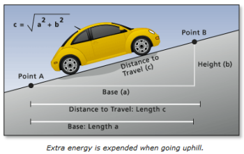
Incorporating directionality through horizontal and vertical factors

Thus far in our cost analysis we have accounted for the cost of travel over the surface using the cost surface and the characters of the mover by applying the source characteristics but we have not yet been concerned with which way the mover is traveling between the regions.

Again, the general cost distance formula is the following:

Cost = Cost of travel    *  Characteristics  *  Movement characteristics
       over the surface     of the mover        on the surface

The Path Distance tool also allows you to account for the Movement characteristics on the surface in the general formula by allowing you to control the direction of travel by the mover through the landscape using the horizontal and vertical factor parameters. Directionality may be important when:

• Locating an escape route for firefighters in an isolated location
• Plotting a secretive course for military troops to reach a sensitive outpost
• Identifying an easy access path between habitat patches for biologists monitoring bobcat populations

Consider the following example of wind as a horizontal factor. Fighting a forest fire into a headwind may be more costly than fighting a fire with the wind at your back. Through the vertical factor, Path Distance also has the capability to adjust for the cost of a traveler to overcome moving uphill versus downhill. Accounting for this vertical factor may play a role in planning for a hiking trail between two remote camp sites.

Hiking trail (blue) from the lower region to the upper region that has the least amount of uphill slopes.

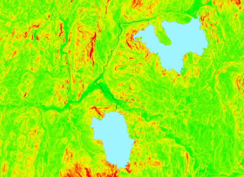
For additional information on the horizontal and vertical factors see How the Horizonal and Vertical factors affect path distance.

Creating corridors

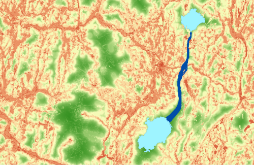
You may want a corridor that is more than one cell wide within which to move between regions. You can use the Buffer tool to create a buffer around the resulting single-cell cost paths described above. However, this buffer would be based on Euclidean distance not accounting for the costs of the locations within the buffer. For instance, a factory maybe included in a wildlife corridor created by the Euclidean buffer which is clearly not desirable. The Corridor tool allows you to create a corridor wider than a single cell based on cost.

Creating a cost corridor is a four step process:

1. Run Cost Distance from the first region.
2. Run Cost Distance from the region you want to connect to.
3. Run Corridor using the cost distance output from steps 1 and 2 above.
4. Use the Extract by Attribute tool to specify the cost threshold that will define the width of the corridor.

Corridors are useful for:

• Outlining a general path firefighters can use to reach a fire in an area without marked trails
• Mapping an area for land troops to stay within to reach a target in case their best route is no longer an option
• Conserving an optimal wildlife corridor for bobcat to move within instead of restricting the animals to a thin pathway when traveling between two habitat patches

Corridor (blue) connecting two bobcat habitat patches.

Conclusion

The two main workflows for cost distance analysis are:

1. Cost distance analysis workflow one: Cost Connectivity - creates an optimum network of paths to connect a series of input patches
2. Cost distance analysis workflow two: Cost Distance/Cost Path - creates individual paths to connect specific sources and destinations

There is synergy between the two workflows allowing you to create the best network of paths for the mover to travel effectively through the landscape.

All workflows for cost distance analysis require a cost surface. Defining the cost units can be difficult, but once this is achieved, the power of creating optimum least-cost solutions is at your fingertips.

Additional cost distance analysis functionality can be used to more accurately capture the movement of the traveler between sources:

1. Use Network Analyst to explore the movement through the resulting network
2. Control the characteristics of the mover and the source from which the mover is moving from
3. Account for the direction of travel by the mover
4. Create corridors instead of single cell paths

The better you can model the movement of the traveler you are interested in, the more effective your decisions will be.

Lessons and resources

The following lessons walk you through the various cost distance analysis workflows to create the optimum network of paths allowing your bobcats to move most deliberately through the Vermont landscape.

Lessons for ArcGIS Desktop

• Lesson 1: Creating a cost surface
• Lesson 2: Creating an optimal connectivity network
• Lesson 3: Creating a least cost path
• Lesson 4: Creating a corridor

Acknowledgements

We thank Steven Lamonde of Johnson State College and the Vermont Center for Geographic Information for their contributions to both the case study and the accompanying lessons.