Available with Spatial Analyst license.
- 1. Data exploration and preprocessing
- 2. Collecting training samples
- 3. Evaluating training samples
- 4. Editing classes
- 5. Creating the signature file
- 6. Clustering (unsupervised classification)
- 7. Examining the signature file
- 8. Editing the signature file
- 9. Applying classification
- 10. Post-classification processing
With the ArcGIS Spatial Analyst extension, the Multivariate toolset provides tools for both supervised and unsupervised classification. The Image Classification toolbar provides a user-friendly environment for creating training samples and signature files used in supervised classification. The Maximum Likelihood Classification tool is the main classification method. A signature file, which identifies the classes and their statistics, is a required input to this tool. For supervised classification, the signature file is created using training samples through the Image Classification toolbar. For unsupervised classification, the signature file is created by running a clustering tool. Spatial Analyst also provides tools for post-classification processing, such as filtering and boundary cleaning. The detailed steps of the image classification workflow are illustrated in the following chart.

1. Data exploration and preprocessing
Data exploration
The classification analysis is based on the assumption that the band data and the training sample data follow normal distribution. To check the distribution of the data in a band, use the interactive Histogram tool  on the Spatial Analyst toolbar. To check the distribution of individual training samples, use the Histograms tool
  on the Training Sample Manager.
Stretching of band data
The classification process is sensitive to the range of values in each band. To have the attributes of each band considered equally, the value range for each band should be similar. If the value range of one band is too small (or too large) relative to the other bands, you can use the mathematical tools in the Spatial Analyst toolbox to stretch it. For example, you can use the Times math tool to multiply the band with a constant value to stretch its value range.
Principal component analysis
Principal component analysis transforms a multiband image to remove correlation among the bands. The information in the output image is mainly concentrated in the first few bands. By enhancing the first few bands, more details can be seen in the image when it is displayed in ArcMap. This could be helpful for collecting training samples. The Principal Components tool from the Multivariate toolset allows you to perform principal component analysis.
Creating a multiband image
The Image Classification toolbar works with a multiband image layer. To load individual bands to a new multiband image, use the Composite Bands tool.
Creating a subset of bands for the classification
To use all bands in an image dataset in the classification, add the image dataset to ArcMap and select the image layer on the Image Classification toolbar.
To use only certain bands from an existing dataset for the classification, create a new raster layer for them using the Make Raster Layer tool. The new raster layer will contain only the specified subset of bands, and can be used in the Image Classification toolbar.
2. Collecting training samples
In supervised classification, training samples are used to identify classes and calculate their signatures. Training samples can be created interactively using the training sample drawing tools on the Image Classification toolbar. Creating a training sample is similar to drawing a graphic in ArcMap except training sample shapes are managed with Training Sample Manager instead of in an ArcMap graphic layer.
To create a training sample, select one of the training sample drawing tools (for example, the polygon tool) on the Image Classification toolbar and draw on the input image layer. The number of pixels in each training sample should not be too small nor too large. If the training sample is too small, it may not provide enough information to adequately create the class signature. If the training sample is too large, you might include pixels that are not part of that class. If the number of bands in the image is n, the optimal number of pixels for each training sample would be between 10n and 100n.

3. Evaluating training samples
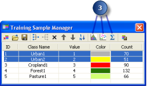
When training samples are drawn in the display, new classes are automatically created in the Training Sample Manager. The manager provides you with three tools to evaluate the training samples—the Histograms tool  , the Scatterplots tool
  , and the Statistics tool
  . You can use these tools to explore the spectral characteristics of different areas. You can also use these tools to evaluate training samples to see if there is enough separation between the classes.

4. Editing classes
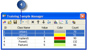
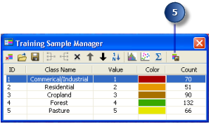
Depending on the outcome of the training sample evaluation, you may need to merge the classes that are overlapping each other into one class. This can be done using the Merge tool  in the manager window. In addition, you can rename or renumber a class, change the display color, split a class, delete classes, save and load training samples, and so forth. The following image shows how to merge two classes:

5. Creating the signature file
Once you determine the training samples are representative of the desired classes and are distinguishable from one another, a signature file can be created using the Create Signature File tool  in the manager window.

6. Clustering (unsupervised classification)
In a supervised classification, the signature file was created from known, defined classes (for example, land-use type) identified by pixels enclosed in polygons. In an unsupervised classification, clusters, not classes, are created from the statistical properties of the pixels. Pixels with similar statistical properties in multivariate space are grouped to form clusters. Clusters have no categorical meaning (for example, land-use type) unlike classes in a supervised classification.
For unsupervised classification using the Image Classification toolbar, the signature file is created by running the Iso Cluster Unsupervised Classification tool. You can also use the Iso Cluster tool from the Multivariate toolset.
The Iso Cluster tool only creates a signature file that can be subsequently used in the classification (step 9 in the above workflow chart). A new tool, Iso Cluster Unsupervised Classification, accessed from both the Image Classification toolbar and the Multivariate toolset, was created to allow you to create the signature file and the output classified image with a single tool (steps 6 and 9).
7. Examining the signature file
The Dendrogram tool allows you to examine the attribute distances between sequentially merged classes in a signature file. The output is an ASCII file with a tree diagram showing the separation of the classes. From the dendrogram, you can determine whether two or more classes or clusters are distinguishable enough; if not, you might decide to merge them in the next step.
The Dendrogram tool is accessible from the Spatial Analyst Multivariate toolset.
8. Editing the signature file
The signature file should not be directly edited in a text editor. Instead, you should use the Edit Signatures tool in the Multivariate toolset. This tool allows you to merge, renumber, and delete class signatures.
9. Applying classification
To classify the image, the Maximum Likelihood Classification tool should be used. This tool is based on the maximum likelihood probability theory. It assigns each pixel to one of the different classes based on the means and variances of the class signatures (stored in a signature file). The tool is also accessible from the Image Classification toolbar.
The Interactive Supervised Classification tool is another way to classify your image. This tool accelerates the maximum likelihood classification process. It allows you to quickly preview the classification result without running the Maximum Likelihood Classification tool.
10. Post-classification processing
The classified image created by the Maximum Likelihood Classification tool may misclassify certain cells (random noise) and create small invalid regions. To improve classification, you may want to reclassify these misclassified cells to a class or cluster that is immediately surrounding them. The most commonly used techniques to clean up the classified image include filtering, smoothing class boundaries, and removing small isolated regions. A more visually appealing map results from the data cleanup tools.
Filtering the classified output
This process will remove single isolated pixels from the classified image. It can be accomplished by either the Majority Filter tool or the Focal Statistics tool with Majority as the statistics type. The difference of the two tools is that the Majority Filter tool assumes a 3 x 3 square neighborhood during the processing, while the Focal Statistics tool supports more neighborhood types (annulus or circle, for example).
Smoothing class boundaries
The Boundary Clean tool clumps the classes and smooths the ragged edges of the classes. The tool works by expanding and then shrinking the classes. It will increase the spatial coherency of the classified image. Adjacent regions may become connected.
Generalizing output by removing small isolated regions
After the filtering and smoothing process, the classified image should be much cleaner than before. However, there may still be some isolated small regions on the classified image. The generalizing process further cleans up the image by removing such small regions from the image. This is a multi-step process which involves several Spatial Analyst tools.
- Run the Region Group tool with the classified image to assign unique values to each region on the image.
- Open the attribute table of the new raster layer created by the Region Group tool. Use the pixel counts to identify the threshold of small regions that you want to remove.
- Create a mask raster for the regions you want to remove. This can be done by running the Set Null tool to set the regions with small numbers of pixels to a null value.
- Run the Nibble tool on the classified image. Use the mask raster created from the Set Null tool from the previous step as the Input mask raster. This will dissolve the small regions on the output image.