Mit der Geostatistical Analyst-Lizenz verfügbar.
With ArcGIS Geostatistical Analyst, you can easily create a continuous surface, or map, from measured sample points stored in a point feature layer or raster layer or by using polygon centroids. The sample points can be measurements such as elevation; depth to the water table; or levels of pollution, as is the case in this tutorial. When used in conjunction with ArcMap, Geostatistical Analyst provides a comprehensive set of tools for creating surfaces that can be used to visualize, analyze, and understand spatial phenomena.
Tutorial scenario
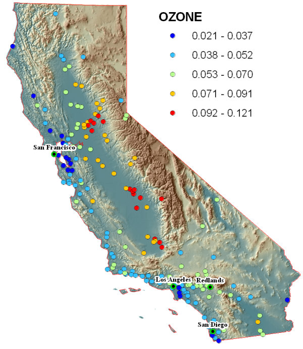
The U.S. Environmental Protection Agency is responsible for monitoring atmospheric ozone concentration in California. Ozone concentration is measured at monitoring stations throughout the state. The locations of the stations are shown here. The concentration levels of ozone are known for all the stations, but the ozone values for other (unmonitored) locations in California are also of interest. However, due to cost and practicality, monitoring stations cannot be placed everywhere. Geostatistical Analyst provides tools that make optimal predictions possible by examining the relationships between all the sample points and producing a continuous surface of ozone concentration, standard errors (uncertainty) of predictions, and probabilities that critical values are exceeded.

The data required to complete the exercises is included on the tutorial data DVD. The tutorial data is also available as a download from the Customer Care website. (You may need to contact the Primary Maintenance Contact at your organization to assist with the download.) When you run the wizard to install this data, check to install the Geostatistical Analyst data (the default installation path is C:\ArcGIS\ArcTutor\Geostatistical Analyst). The following datasets (which are contained in a geodatabase called ca_ozone.gdb) will be used in the tutorial:
| Dataset | Description |
|---|---|
ca_outline | Outline of California |
O3_Sep06_3pm | Ozone point sample values (ppm) |
ca_cities | Major California cities |
ca_hillshade | A hillshade map of California |
The ozone dataset (O3_Sep06_3pm) was provided courtesy of the California Air Resources Board and represents the concentration of ozone measured on September 6, 2007 between 3:00 and 4:00 p.m. in parts per million (ppm). The original data has been modified for the purpose of the tutorial and should not be considered accurate data.
From the ozone point samples (measurements), you will produce two continuous surfaces (maps) predicting the values of ozone concentration for every location in the state of California. The first map that you create will simply use all the default options to introduce you to the process of creating a surface from your sample points. The second map that you produce will allow you to incorporate more of the spatial relationships that are discovered among the points. When creating this second map, you will use the exploratory spatial data analysis (ESDA) tools to examine your data. You will also be introduced to some of the geostatistical options that you can use to create a surface, such as removing trends and modeling spatial autocorrelation. By using the ESDA tools and working with the geostatistical parameters, you will be able to create a more accurate surface. Many times, it is not the actual values of some critical health risk that are of concern but rather whether the values are above some toxic level. If this is the case, immediate action must be taken. The third surface you create will assess the probability that a critical ozone threshold value has been exceeded. For this tutorial, the critical threshold will be if the value of ozone goes above 0.09 ppm (California State's ambient air quality standard for hourly measurements); then the location should be closely monitored. You will use Geostatistical Analyst to predict the probability that ozone values across California complied with this standard on September 6, 2007 between 3:00 and 4:00 p.m.
This tutorial is divided into individual tasks that are designed to let you explore the capabilities of Geostatistical Analyst at your own pace.
- Exercise 1 takes you through accessing Geostatistical Analyst and the process of creating a surface of ozone concentration using default parameter values to introduce you to the steps involved in creating an interpolation model.
- Exercise 2 guides you through the process of exploring your data before you create the surface to spot outliers and recognize trends.
- Exercise 3 creates a second surface that incorporates more of the spatial relationships discovered in exercise 2 and improves on the surface you created in exercise 1. This exercise also introduces you to some of the basic concepts of geostatistics.
- Exercise 4 shows you how to compare the results of the two surfaces that you created in exercises 1 and 3 and how to decide which surface provides the better predictions of the unknown values.
- Exercise 5 takes you through the process of mapping the probability that ozone exceeded a critical threshold, creating a third surface.
You will need a few hours of focused time to complete the tutorial. However, you can also perform the exercises one at a time if you want. It is recommended that you save your results after each exercise.