Mit der Geostatistical Analyst-Lizenz verfügbar.
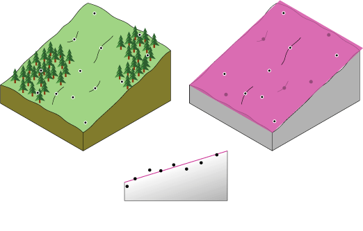
In Analyzing the surface properties of nearby locations, interpolation that depends on distance was presented. There are other solutions for predicting the values for unmeasured locations. Another proposed site for the observation area is on the face of a gently sloping hill. The face of the hill is a sloping plane. However, the locations of the samples are in slight depressions or on small mounds (local variation). Using the local neighbors to predict a location may over- or underestimate the prediction because of the influence of depressions and mounds. Further, you might pick up the local variation and may not capture the overall sloping plane (referred to as the trend). The ability to identify and model local structures and surface trends can increase the accuracy of your predicted surface.
Global polynomial interpolation
To base your prediction on the overriding trend, you can fit a plane between the sample points. A plane is a special case of a family of mathematical formulas called polynomials. You then determine the unknown height from the value on the plane for the prediction location. The plane may be above certain points and below others. The goal for interpolation is to minimize error. You can measure the error by subtracting each measured point from its predicted value on the plane, square it, and add them. This sum is referred to as a least-squares fit. This process is the theoretical basis for first-order global polynomial interpolation.

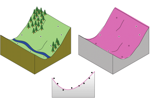
But what if you were trying to fit the plane to a landscape that is a valley? You will have a difficult task obtaining a good surface from a plane. However, if you are allowed one bend in the plane, you might be able to obtain a better fit (get closer to more values). To allow one bend is the basis for second-order global polynomial interpolation (see below). Two bends in the plane would be a third-order polynomial, and so forth. The bends can occur in both directions, possibly resulting in a bowl-shaped surface.
