Mit der Geostatistical Analyst-Lizenz verfügbar.
In most GIS literature, areal interpolation specifically means the reaggregation of data from one set of polygons (the source polygons) to another set of polygons (the target polygons). For example, demographers frequently need to downscale or upscale the administrative units of their data. If population counts were taken at the county level, a demographer may need to downscale the data to predict the population of census blocks. In the case of large-scale redistricting, population predictions may be needed for a completely new set of polygons.
Areal interpolation in the Erweiterung "ArcGIS Geostatistical Analyst" is a geostatistical interpolation technique that extends kriging theory to data averaged or aggregated over polygons. Predictions and standard errors can be made for all points within and between the input polygons, and predictions (along with standard errors) can then be reaggregated back to a new set of polygons.
Other kriging methods in Geostatistical Analyst require point data that is continuous and Gaussian, but areal interpolation allows polygonal data to be discrete counts. A second set of polygons can also be used as a cokriging variable; these secondary polygons can have identical geometry to the polygons of the primary variable, or the polygons can be completely different.
Polygon-to-polygon data reaggregation workflow
Reaggregating polygonal data (for example, downscaling population counts) is a two-step process. First, a smooth prediction surface for individual points is created from the source polygons (this surface can often be interpreted as a density or risk surface), then the prediction surface is aggregated back to the target polygons. Creating the prediction surface requires interactive variography, so it must be done in the Geostatistical Wizard. The output from the Geostatistical Wizard is a geostatistical layer of predictions or prediction standard errors. If reaggregation to new polygons is not required, the workflow can end here.
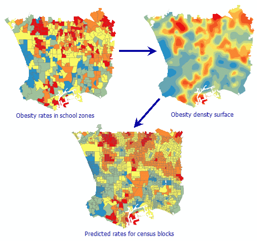
Once a prediction surface has been created, aggregation back to a different set of polygons is done with the Areal Interpolation Layer To Polygons tool. The graphic below shows the workflow for predicting obesity rates in Los Angeles census blocks from obesity rates in Los Angeles school zones.

The mathematical details of the disaggregation and reaggregation can be found in the paper referenced at the end of this topic.
What types of data can be used in areal interpolation?
Areal interpolation accepts three different polygonal dataset types as input. All three can produce prediction and standard error surfaces and can then be reaggregated to target polygons. The interpretations of the prediction surfaces and the reaggregated predictions are different for each data type, as described below.
Average (Gaussian) data
To protect privacy or reduce overhead, continuous point measurements are sometimes averaged over areal regions, and the original point data is discarded or kept private. For example, average pollution levels for counties may be reported, but the individual point measurements may be kept private. Without knowing where the pollution was measured, other kriging methods are not appropriate.
Areal interpolation for continuous data requires that the data is Gaussian and averaged over defined polygons. Given the polygons and the average measurements, a prediction (or standard error) surface is produced for the value of the Gaussian variable at all points in the data domain.
Inputs
- Source Dataset—Specify the polygon features.
- Value Field—Specify the average value for each polygon from the source dataset.
For Gaussian areal interpolation, the Areal Interpolation Layer To Polygons tool predicts the average value of the Gaussian variable (with prediction standard errors) for the target polygons. For example, given the average temperature of all counties in a state for a particular day, the average temperature for cities within the counties can be predicted.
Rate (binomial) counts
A typical source of polygonal data is when individuals are randomly sampled from the population within a polygon, and the number of individuals with a particular characteristic is counted (this is called binomial sampling). The value of interest is the proportion of sampled individuals that have the characteristic.
Given the number of individuals sampled and the number of individuals with the characteristic for each polygon, areal interpolation for binomial counts produces a risk prediction surface (or standard error surface) for all points in the data domain. The risk at any individual point represents the probability that an individual sampled at that location will have the characteristic.
For example, a company might want to ask some of its clients whether they are happy with the service that the company provides. In this case, the characteristic of interest is that the client is happy with the service. The exact locations of the sampled clients may not be known; the company may only know their geographic region (such as city or area code). Areal interpolation for binomial counts produces a map showing locations of high and low support for the company. The company can then do further research to find out why clients from certain locations are happier with its service than clients from other locations.
For accurate predictions, the samples must be taken randomly. Every member of the population of a polygon must have the same probability of being chosen for the sample. If preference is shown for particular individuals, the predictions will be biased.
Inputs
- Source Dataset—Specify the polygon features.
- Count Field—Specify the field with the number of individuals with a specific characteristic for each polygon.
- Population Field—Specify the field with the number of individuals sampled for each polygon.
For binomial areal interpolation, the Areal Interpolation Layer To Polygons tool predicts the proportion of individuals with the characteristic for each specified polygon. For example, if the number of lung cancer cases for each county in a state is known (along with the population at risk in each county), the proportion of individuals with lung cancer can be predicted for postal codes within the counties. To get an estimate of the number of lung cancer cases in each postal code, multiply the predicted proportion of lung cancer cases by the population of each postal code. Similarly, multiplying the standard errors by the population of each postal code gives the standard error for the predicted number of lung cancer cases in each postal code.
Event (overdispersed Poisson) counts
Another common source for polygonal data is when the number of instances of a certain event is counted within a defined area for a specified amount of time. For example, whale watchers collect their data by sailing around defined areas in the ocean and counting the number of whales that they see. In this case, an event would be the sighting of a whale. Because the number of whales observed is assumed to be proportional to how long the whale watchers were watching, it is necessary to record the amount of time they spent counting. For each expedition, the whale watchers will know the viewing polygon (the area where they watched), the number of events witnessed (number of whales seen), and the time they spent observing.
Areal interpolation for event counts produces a surface that predicts the underlying risk of witnessing an event at a specific location. A higher risk means that there is a higher chance of witnessing an event at that location. In the case where the event is finding a physical object (like a whale), the prediction surface can be interpreted as a density map.
For most use cases, the observation time for each polygon will be the same. For example, crime statistics frequently come in the form of counts for a single year for each polygon. Because a constant observation time is so common, if the observation time is not specified, the software assumes that counts were taken in a single unit of time for each polygon. In the case of a complete census (where every event is witnessed, such as a total population count), the observation time for each polygon should be assumed to be the same.
When observing, it is not necessary to witness every single event. It is only necessary that the number of events witnessed per unit of time is proportional to the underlying density of whatever is being observed. In practice, this means that the methodology used for making observations needs to be roughly the same for each polygon. For example, if a whale watcher from one expedition is more skilled at spotting whales than a watcher from another expedition, the predictions will be biased.
Inputs
- Source Dataset—Specify the polygon features.
- Count Field—Specify the field with the number of events witnessed in each polygon.
- Time Field—Optionally, specify the amount of time spent counting in each polygon. If the field is left blank, the software assumes that all counts were taken in one unit of time.
For overdispersed Poisson areal interpolation, the Areal Interpolation Layer To Polygons tool predicts the number of counts per unit time for each specified polygon. For example, if the whale watchers recorded their observation times in hours, the prediction for a new polygon is interpreted as the expected number of whales that will be observed in that polygon in a single hour. For census population data, the interpretation is simply the predicted population of the polygon at the time of the census.
Building a valid model
As with all geostatistical interpolation methods, the accuracy of your predictions in areal interpolation depends on the accuracy of your model. With this in mind, much care should be taken to build a valid model within the Geostatistical Wizard.
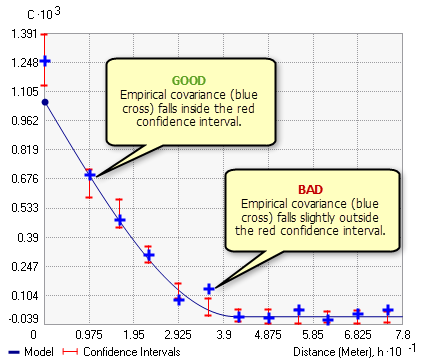
Because areal interpolation in the Erweiterung "ArcGIS Geostatistical Analyst" is implemented through a kriging framework, interactive variography is an essential step in building the model. It is often difficult to visually judge the quality of a covariance curve, so confidence intervals (the red vertical lines in the graphic below) are provided for each empirical covariance (blue crosses). If the covariance model is properly specified, you expect 90 percent of the empirical covariances to fall within the confidence intervals. In the graphic below, 11 of the 12 empirical covariances fall within the confidence intervals, and 1 point falls a bit outside the confidence interval. This indicates that the model fits the data, and the results can be trusted.

The default covariance curve often does not fit the data well. In this case, the variography parameters on step 2 of the Geostatistical Wizard need to be altered. Fitting a proper covariance curve is often difficult, and the best way to get better at fitting is simply to practice, but there are a few rules of thumb that can help to fit a good model:
- Decrease the Lag Size value until the empirical covariances are no longer negative.
- If the model still doesn't fit, experiment with the Type parameter. K-Bessel and Stable are the most functional models, but they also take the longest to process.
- If you find a combination of Lag Size and Type that nearly fits, try decreasing the Lattice Spacing value. However, be aware that decreasing the lattice spacing will rapidly increase the processing time. The lattice spacing parameter is described in the "New parameters for areal interpolation" section below.
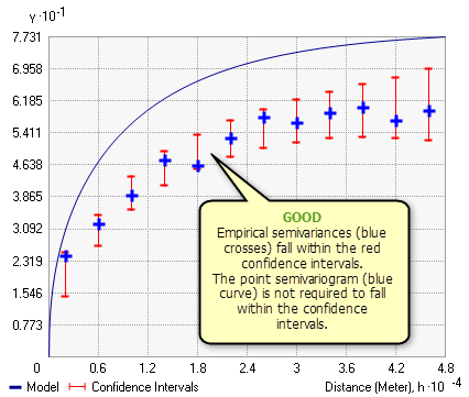
As seen in the graphic below, if Variable is changed to Semivariogram on step 2 of the Geostatistical Wizard, the semivariogram curve for points (the blue line in the graphic below) might not pass through the confidence intervals. This is not a problem, and the criteria for a good model does not change: if a large percentage of the empirical semivariances fall within the confidence intervals, you can be confident in the accuracy of your model.

New parameters for areal interpolation
In the Geostatistical Wizard, you will encounter three parameters that do not appear in other kriging methods:
- Lattice Spacing—To estimate point covariances, each polygon is overlaid with a square lattice, and a point is assigned to each intersection in the lattice. The lattice spacing parameter specifies the horizontal and vertical distance between each point. If the lattice spacing is large enough that a polygon does not receive a point, a point is placed at its centroid. A smaller lattice spacing will make predictions more precise, but it will also increase processing time. For example, cutting the lattice spacing in half will take four times longer to process.
- Confidence Level—Specifies the confidence level for the confidence intervals for the semivariogram/covariance curves. If the model is correct, this value indicates the percentage of empirical covariances/semivariances that should fall within the confidence intervals. Note that the point semivariogram line will not necessarily fall within the confidence intervals. This parameter is for diagnostic purposes only; the value will not affect predictions.
- Overdispersion Parameter—Only applicable for event (overdispersed Poisson) count data. In Poisson count data, overdispersion (greater variability than is expected from the Poisson model) is frequently observed. The overdispersion parameter helps correct this. The parameter is equal to the inverse of the dispersion parameter of the negative binomial distribution.
All other parameters have the same meaning as in other kriging methods.
Limitations
As with all kriging methods, areal interpolation comes with several limitations that may prevent you from finding a valid model for your data.
Nonstationarity
One of the most stringent kriging assumptions is the assumption of data stationarity. Stationarity is the assumption that the statistical relationship between any two polygon data values depends only on the distance between the polygons. For example, human populations often cluster into cities with few people living in the areas between cities. This is problematic for areal interpolation because under stationarity, the population density should change smoothly across the landscape; you should not see extremely dense populations right next to extremely low population densities. For nonstationary data like this, fitting a valid areal interpolation model will be very difficult, if not impossible.
Polygons of vastly different sizes
If some of your polygons have very small areas compared to the largest polygons, the software may fail to differentiate the smallest polygons, and it will treat them as coincident polygons. This can happen because the lattice spacing parameter discretizes the polygons, and more than one polygon may be represented as a single point in the lattice. This will result in an error because areal interpolation does not support coincident polygons. To resolve this error, follow these steps:
- Use the Find Identical and Delete Identical tools to locate and delete the coincident polygons. If no coincident polygons are detected or the removal does not resolve the error, proceed to the next step.
- Manually lower the lattice spacing until the software is able to differentiate the polygons. However, lowering the lattice spacing rapidly increases calculation time. If you find that the required lattice spacing takes too long to process, proceed to the next step.
- Deselect the smallest polygons in your feature class so that they are not used in the calculation.
References
- Krivoruchko, K., A. Gribov, E. Krause (2011). "Multivariate Areal Interpolation for Continuous and Count Data," Procedia Environmental Sciences, Volume 3: 14–19.