Aloha! A GIS vacation

Note:

This example use case presents an approach to using ArcGIS to perform three-dimensional surface analysis. While the data is real, the scenario, analysis, and resulting decisions are hypothetical.

The primary objective of this case study is to demonstrate surface analysis and 3D display of rasters. The workflow includes tools such as Topo to Raster, Hillshade, Viewshed, Slope, Focal Statistics, and the Raster Calculator. The workflow also introduces creating tools in ModelBuilder.

The workflow requires access to ArcGIS 3D Analyst extension and ArcGIS Spatial Analyst extension. If you do not have access to 3D Analyst you can also complete the workflow in 2D using Spatial Analyst.

A GIS vacation

A GIS analyst is on vacation in Hawai'i! She is planning her last day on O'ahu and needs to decide between two lookout points known for their panoramic views: Diamond Head crater and the Nu'uanu Pali lookout. Like all GIS analysts, she has brought her laptop on vacation and decides to research the areas and model the scenes from the lookouts to make her decision easier. Her research and workflow are outlined below.

The two lookout locations displayed in a 3D Scene in ArcGIS Pro

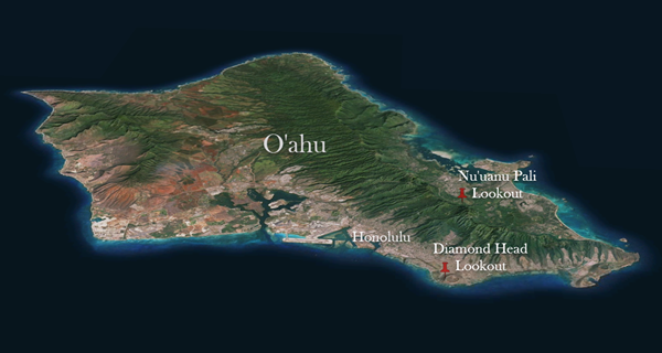
Diamond Head State Monument

Diamond Head (Lē'ahi in Hawai'ian) is a crater located adjacent to Waikīkī Beach and was formed 300,000 years ago through an explosive volcanic eruption. The crater has been used by the United States military as a lookout point and a trail was built to the summit in 1908. The hiking trail, which ascends the inner face of the crater, is now open to the public. The summit of Diamond Head includes old military bunkers and lookout spots with a view of Waikīkī.

A view of Diamond Head crater from Waikīkī Beach

Nu'uanu Pali lookout

The Nu'uanu Pali lookout is a scenic lookout on O'ahu’s Windward Coast with important historical significance for the Hawai'ian Islands. King Kamehameha of the Big Island had a vision to unite the Hawai'ian islands under one monarchy. In 1795, after he had already conquered Maui, Moloka'i, and Lāna'i, King Kamehameha and his army traveled to O'ahu, where they invaded the shores near Waikīkī. The ensuing battle ended on the Nu'uanu cliffs, where King Kamehameha’s army advanced and forced the O'ahu army off the cliffs. Today, the site is a popular tourist attraction because of its historical importance and its panoramic view of the Windward Coast, including the towns Kāne'ohe and Kailua.

A view from the Nu'uanu Pali lookout

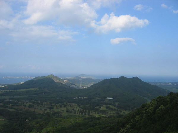
The view from the top

The analyst uses 3D Scenes to explore the areas around the lookout locations to learn more about the views. Both lookouts give an elevated view of the Ko'olau Range and the ocean, but Diamond Head overlooks Waikīkī, whereas Nu'uanu Pali overlooks Kāne'ohe.

The Nu'uanu Pali lookout overlooks the town of Kāne'ohe on the Windward Coast of O'ahu.

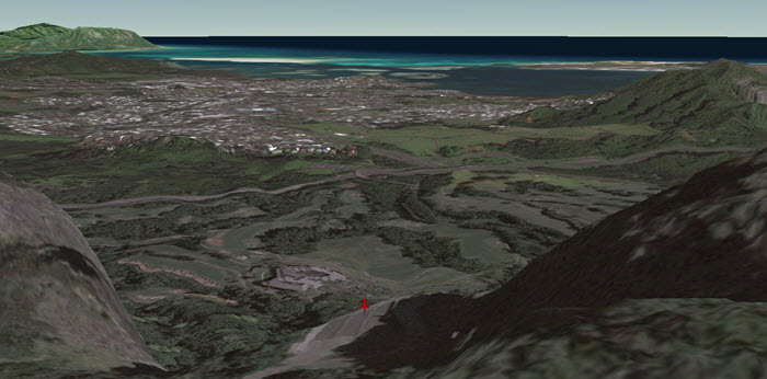
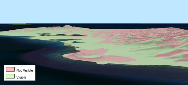
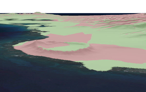
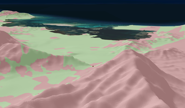
To get a more exact representation of the views, the analyst decides to create viewsheds for each lookout so she will know exactly which features on the island will fall within her sight range. A larger area of the island is visible from Diamond Head than from Nu'uanu Pali.

The viewshed from Diamond Head shows that there is a view of both mountain ranges as well as most of Honolulu.

Determining hiking difficulty

One of the main differences to consider when choosing between the two tourist sites is that the Nu'uanu Pali lookout is accessible by car, but you must hike to reach the summit of Diamond Head. The analyst uses the elevations to determine the slopes on the island.

The changes in slope, or ruggedness, can also be used to determine hiking difficulty. The Topographic Position Index (TPI) can be used to determine which areas are a valley, a ridge, or flat and can be applied to an area using the elevation for each cell and subtracting the average elevation of the cell’s neighbors (Weiss, 2001):

TPIpt = Hpt - µpt 
 where:
	Hpt = elevation at point pt
	µpt = mean elevation in the neighborhood of point pt

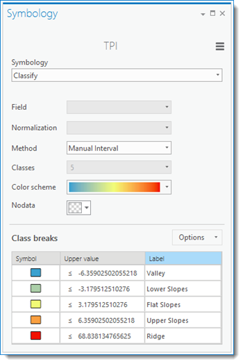
The Standard Deviation (σ) of the TPI values can be used to apply qualitative descriptions to the data:

• Valley < -1σ
• -1σ ≤ Lower Slopes ≤ -0.5σ
• -0.5σ ≤ Flat Slopes ≤ 0.5σ
• 0.5σ ≤ Upper Slopes ≤ 1σ
• Ridge ≥ 1σ

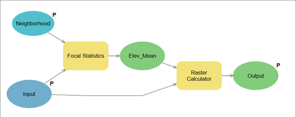
A tool was built to profile the crater based on the TPI using ModelBuilder. The tool can be used with any elevation dataset.

A model used to determine the ruggedness of the Diamond Head crater based on the TPI.

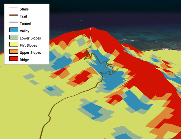
Finally, the analyst compares the slopes and TPI designations to a feature class she has made of the trail. She can tell that the trail was mostly built on areas with lower slopes and that it zigzags through valleys and ridges or uses stairs to ascend in steep areas.

The ruggedness of Diamond Head is based on the TPI. The hiking trail zigzags through valleys and over ridges.

Workflow using ArcGIS Desktop

Note:

The steps below are based on ArcGIS Desktop 10.4, but should also be accurate for newer versions. The data is available for ArcGIS Desktop versions 10.1, 10.3, and 10.4. The workflow requires access to ArcGIS 3D Analyst extension and ArcGIS Spatial Analyst extension, but can also be completed in 2D using Spatial Analyst only.

The data can be accessed in the form of a layer package using the Download the data button at the top of the page. Use the Extract Package tool in ArcScene or ArcMap to unpack the data. Use the Catalog window to browse to your data and add the layers to your Map or Scene. You may want to add the feature classes, rather than the layer files for easier processing. You may also want to apply the layer symbology to the Lookouts and TrailLine feature classes. Turn off all of the layers except for the imagery and Lookouts.

Prepare data to be used in 3D

1. Elevation data (in feet) was found in a 2D contour dataset. In order to use the elevation values, the layer's projection needs to be in feet. Set the Scene's coordinate system to a Hawai'i State Plane projection that uses feet, rather than degrees or meters:
   • Open the Scene Properties dialog box by double clicking Scene Layers.
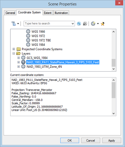
   • Go to the Coordinate System tab. If the Current coordinate system is not already set to NAD_1983_PA11_StatePlane_Hawaii_3_FIPS_5103_Feet, then go to the Layers folder and expand the Hawaii State Plane projection. The Lookouts, TrailLine, and Extent layers are using the Hawai'i State Plane projection. Click the projection to highlight it and click OK.

   

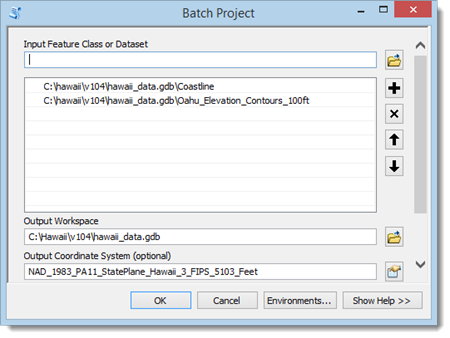
2. Use Batch Project to project the contours and coastline to the same Hawai'i State Plane projection. Replace the layers in the scene with the projected feature classes.

   

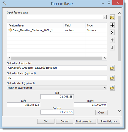
3. Contours cannot be used as input for many of the 3D Analyst tools. Therefore, the contours need to be converted to rasters. Use the Topo to Raster tool to create an elevation raster. It may take several minutes for the tool to finish running.

   Tip:

   It is important to set the Environment Settings for your map document when working with raster data. Set the Extent to Same as layer Extent, the Cell Size to 50 and the Mask to Coastline_1 (the projected coastline feature class.) You can also set your Scratch Workspace to your current folder.

   

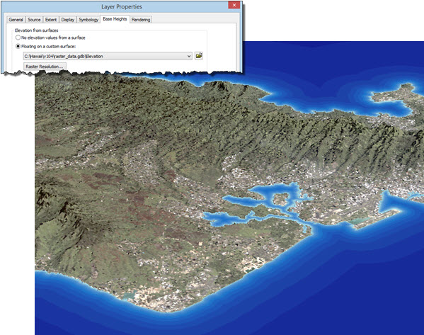
4. Now that you have an elevation raster you can display your data in 3D. Right-click the satellite image of O‘ahu and open the Layer Properties dialog box. Go to the Base Heights tab and check Floating on a custom surface. Make sure the elevation raster is chosen in the drop down. Repeat the process for the Lookouts, choosing the elevation raster again. Turn off all of the layers except for the lookouts and the satellite image. You may also want to set the Scene's Vertical Exaggeration to 1.5.

   

   Tip:

   The Multiple Ring Buffer tool was used to create the shoreline effect seen above. Read the Symbolizing shorelines blog to find out how.

Analyze views from two lookout points

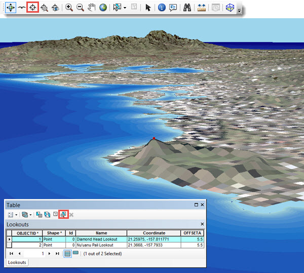
1. The analyst wants to use the imagery and elevation data to get familiar with the areas around the lookouts. Open the Lookouts attribute table, highlight the Diamond Head lookout, and choose Zoom to Selected Feature. You may have to zoom out on the scene to see the selected lookout. Click the Center on Target tool and click the lookout pin. The axis of rotation for the scene is now at the lookout location. Use the Explore tool to rotate the scene around and see the view from Diamond Head. Repeat the process for the Nu'uanu Pali Lookout.

   

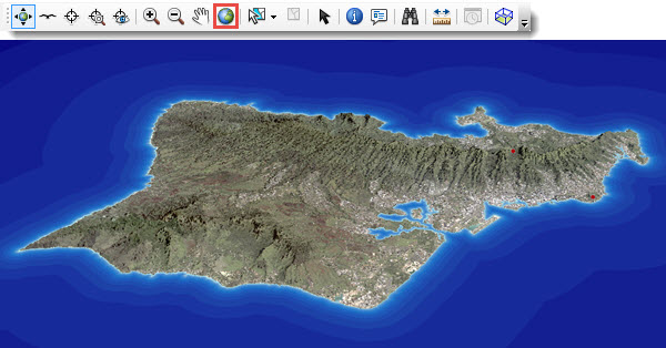
2. Reset the axis of rotation by zooming to the full extent of the scene.

   

Create viewsheds from the lookouts

1. Hillshades are useful for making visually appealing maps with elevation data in 2D and 3D. Use the Hillshade tool to create a Hillshade raster.

   

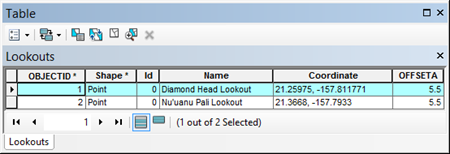
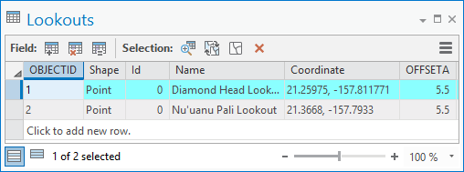
2. The analyst wants to make a Viewshed raster for each lookout. Open the Lookouts attribute table and select the Diamond Head lookout. Any tools you run with the Lookout layer will only use the selected row. The OFFSETA field will be used to apply the analyst's height (5' 6") to the Viewshed analysis.

   

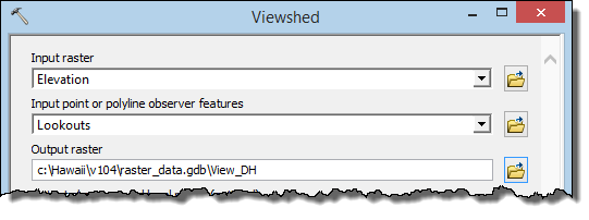
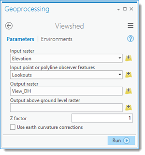
3. Use the Viewshed tool to create Viewsheds from the lookout. Use the elevation raster as the input raster.

   

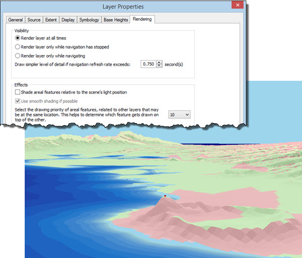
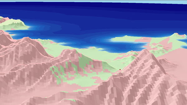
4. The Viewshed tool classifies each cell as being visible (green) or not visible (pink) based on the elevation raster and the location of the observer points. Set the Base Height of the Viewshed and the Hillshade to the elevation raster and the transparency of the Viewshed to 30 percent. Display the Viewshed layer over top of the Hillshade. You may need to change the drawing priority of the Hillshade (under the Rendering tab) to get the layers to display properly together.

   

Tip:

You can set the layer transparency in the Display tab of the Layer Properties dialog box.

5. Repeat steps 1-3 above with the Nu'uanu Pali lookout.

   

Determining the visible area

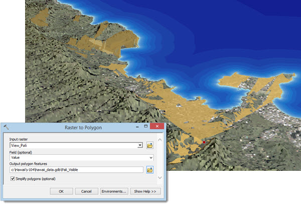
1. The analyst wants to know the total land area that is visible from each lookout, but the tools that calculate area will not use rasters as input. Therefore, she will convert the rasters to polygons before calculating the area. Open the attribute table of the Nu'uanu Pali Viewshed and select the row with a Value of 1 (visible cells). Use the Raster to Polygon tool to create a feature class out of the selected raster cells.

   

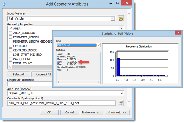
2. Calculate an area field (square miles) using Add Geometry Attributes. Calculate the total visible area using Statistics.
   • There are just under 17 square miles of land visible from the Nu'uanu Pali lookout.

   

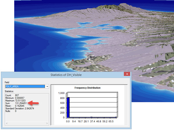
3. Repeat steps 1 and 2 above for the Diamond Head lookout.
   • There are over 131 square miles of land visible from Diamond Head.

   

Profiling the Diamond Head hiking trail

Diamond Head is closer to the analyst's hotel and gives a view of more of the island than the Nu'uanu Pali Lookout. However, the Nu'uanu Pali lookout is accessible by car, whereas Diamond Head must be hiked. After seeing the inner face of the crater, she decides to analyze the slope and ruggedness around the hike to the summit before making a decision.

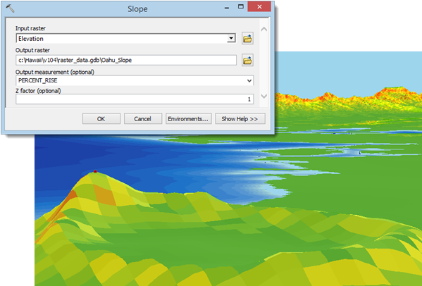
1. Use the Slope tool to find out more about the crater.

   

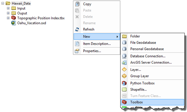
2. A Topographic Position Index can be used to determine ruggedness of terrain. The TPI can be calculated by comparing each cell slope value to the mean slope of the cell's neighbors. A model tool will be created to perform this analysis. A toolbox must be created to store the model tool. Create a toolbox for your model in your home folder.

   Note:

   Calculations and classifications for TPI were based on an algorithm presented by Andrew D. Weiss of the Nature Conservancy (Weiss, 2001). The model created in this section is based on a tool created by Tom Dilts of the University of Nevada Reno (Dilts, 2016).

   

3. Open ModelBuilder using the Standard toolbar. Set the Model Properties and save the blank model in your toolbox.

   

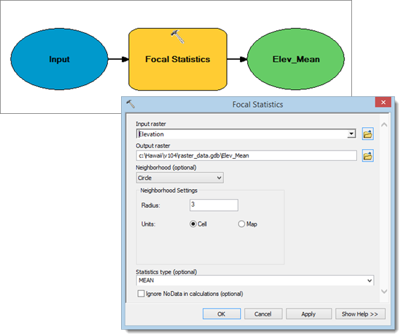
4. The Focal Statistics tool can be used to calculate the mean cell value in raster neighborhoods. Add the Focal Statistics tool to the model and fill in its parameters so that the tool calculates the mean cell value of neighborhoods with a radius of three cells. Rename the Elevation bubble as Input.

   

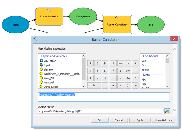
5. The Raster Calculator will be used to subtract the mean cell values from the original cell values. Add the Raster Calculator to the model and enter the following expression:"%Input%"–"%Elev_Mean%"

   

6. In order to make the model a stand-alone tool, some of the tool parameters should be editable. Make a variable in the Focal Statistics tool out of the Neighborhood parameter.

   

7. Make model parameters out of the Input, Neighborhood and TPI elements by right-clicking their bubbles and checking Model Parameter. Those elements will show up as tool parameters when the tool is run. Rename TPI as Output. Save and close the model.

   

8. Now that the model is complete, the tool must be documented. Open ArcCatalog and navigate to your model. Choose Edit from the Description tab.

   

9. Create entries for the Tags, Summary, and Usage sections as well as help entries for the Input, Output, and Neighborhood parameters. Save the edits and exit ArcCatalog.

   

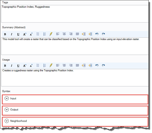
10. In ArcScene, double-click your model to open up the tool. Click Show Help to see the help items you entered in ArcCatalog. Click OK to run the model as a tool.

    

    Tip:

    If an error occurs when running your tool, try changing the output format to a TIFF.

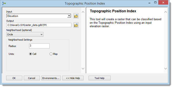
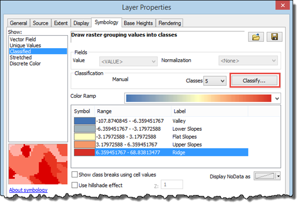
11. In order to view the data correctly for the TPI the analyst must change the layer's symbology. In the TPI Layer Properties dialog box, go to Symbology and change the symbology type to Classified. If you are asked to make a histogram, click OK. Open up the Classification dialog by clicking Classify… and change the method to Standard Deviation. Use the Break Values to determine the standard deviation (σ) of your data. Note that the last break value may represent the highest data value and may not be useful for calculating σ. Change the Classification Method to Manual and the number of Classes to 5. Leave the last break, but change the first to fourth breaks to -1σ, -0.5σ, 0.5σ, and 1σ respectively. Change the Label values as seen in the dialog box below.

    

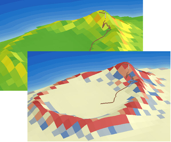
12. Turn on the Diamond Head trail layer that the analyst digitized and note the slope and TPI in the area around the trail. The trail winds up the crater and avoids the steepest areas by using a zigzag pattern to ascend through valleys and ridges.

    

    The analyst decides that the hike will not be as difficult as choosing between Diamond Head and the Nu'uanu Pali lookout. Doing the 3D analysis was so exciting that she decides to get up early in the morning and visit both attractions.

Workflow using ArcGIS Pro

Note:

The steps below are based on ArcGIS Pro 1.2, but should also be accurate for newer versions. The workflow requires access to ArcGIS 3D Analyst extension and ArcGIS Spatial Analyst extension. If you do not have access to 3D Analyst, the workflow can be completed using Spatial Analyst only.

The data can be accessed in the form of a layer package using the Download the data button at the top of the page. Create a new blank Scene and use the Extract Package tool in ArcGIS Pro to unpack the data. Use the Project pane to browse to your data and add the layers to your Scene. You may want to add the feature classes rather than the layer files for easier processing. You may also want to apply the layer symbology to the Lookouts and TrailLine feature classes. If you would like to use one of the 3D Basemaps rather than the provided TIFF file, you may add or change the Basemap in the Map tab. Turn off all of the layers except for the imagery and the Lookouts.

For more information on finding geoprocessing tools, using the Project pane, navigating a 3D scene, and other topics, please see the ArcGIS Pro Help page.

Prepare data to be used in 3D

1. Elevation data (in feet) was found in a 2D contour dataset. In order to use the elevation values, the layer's projection needs to be in feet. Set the Scene's coordinate system to a Hawai'i State Plane projection that uses feet, rather than degrees or meters.
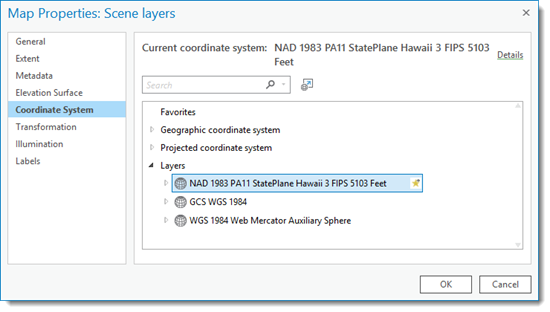
   • Open the Scene Properties dialog box by double-clicking Scene Layers.
   • Go to the Coordinate System tab. If the Current coordinate system is not already set to NAD_1983_PA11_StatePlane_Hawaii_3_FIPS_5103_Feet, then go to Layers and expand the Hawai'i State Plane projection. The lookouts, trails, and extent layers are using the Hawai'i State Plane projection. Click the projection to highlight it and click OK.

   

2. Use Batch Project to project the contours and coastline to the same Hawai'i State Plane projection. Replace the feature classes in the scene with the projected feature classes.

   Tip:

   If you are unable to browse to your data, make a folder connection to the inputs and drag and drop the files into the Input Feature Class or Dataset parameter.

   

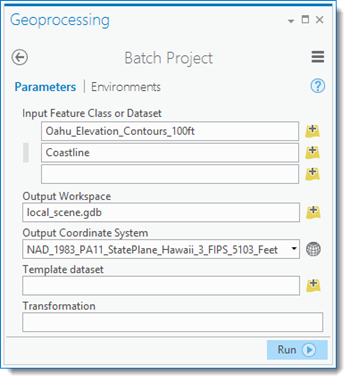
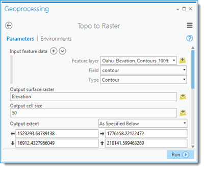
3. Contours cannot be used as input for many of the 3D Analyst tools. Therefore, the contours need to be converted to rasters. Use the Topo to Raster tool to create an elevation raster. It may take several minutes for the tool to finish running.

   Tip:

   It is important to set the Environment Settings for your map document when working with raster data. Set the Extent to Same as layer Extent, the Cell Size to 50 and the Mask to Coastline. You can also set your Scratch Workspace to your current folder.

   

Analyze views from two lookout points

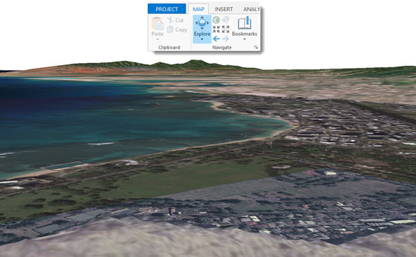
1. The analyst wants to use the Basemap imagery and elevation to get familiar with the areas around the lookouts. Use the Explore tool to explore the scene. You can pan by left-clicking and dragging the scene or zoom in and out by holding down the right button and moving the mouse up and down or scrolling. The spot where you first click becomes the center of rotation. Repeat the process for the Nu'uanu Pali lookout.

   

Create viewsheds from the lookouts

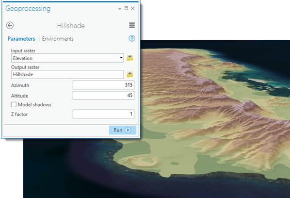
1. Hillshades are useful for making visually appealing maps with elevation data in 2D and 3D. Use the Hillshade tool to create a Hillshade raster. Move the Hillshade to just above the Imagery Basemap and set the transparency of the Elevation to 30 percent.

   

Tip:

You can set the layer transparency of the selected layer in the Effects group of the Appearance tab.

2. The analyst wants to make a Viewshed raster for each lookout. Open the Lookouts attribute table and select the Diamond Head lookout. Any tools you run with the Lookout layer will only use the selected row. The OFFSETA field will be used to apply the analyst's height (5' 6") to the Viewshed analysis.

   

3. Use the Viewshed tool to create Viewsheds from the lookout. Use the elevation raster as the input raster.

   

4. The Viewshed tool classifies each cell as being visible (green) or not visible (pink) based on the elevation raster and the location of the observer points. Display the Viewshed layer over top of the Hillshade and set the transparency to 30 percent.

   

5. Repeat steps 1-3 above with the Nu'uanu Pali lookout.

   

Determining the visible area

1. The analyst wants to know the total land area that is visible from each lookout, but the tools that calculate area will not use rasters as input. Therefore, she will convert the rasters to polygons before calculating the area. Open the attribute table of the Nu'uanu Pali Viewshed and select the row with a Value of 1 (visible cells). Use the Raster to Polygon tool to create a feature class out of the selected raster cells.

   

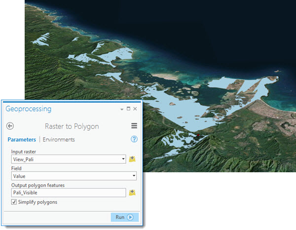
2. Calculate an area field (square miles) using Add Geometry Attributes. Calculate the total visible area using Summary Statistics.
   • There are just under 17 square miles of land visible from the Nu'uanu Pali lookout.

   

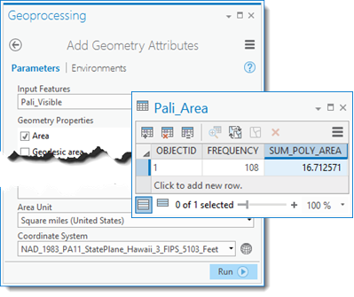
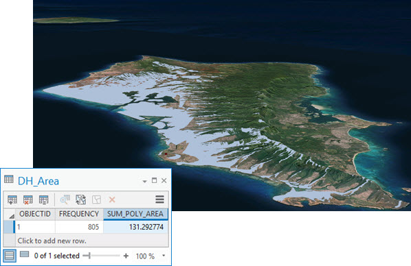
3. Repeat steps 1 and 2 above for the Diamond Head lookout.
   • There are over 131 square miles of visible land from Diamond Head.

   

Profiling the Diamond Head hiking trail

Diamond Head is closer to the analyst's hotel and gives a view of more of the island than the Nu'uanu Pali lookout. However, the Nu'uanu Pali lookout is accessible by car, whereas Diamond Head must be hiked. After seeing the inner face of the crater, she decides to analyze the slope and ruggedness around the hike to the summit before making a decision.

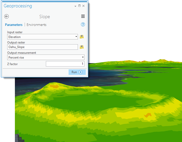
1. Use the Slope tool to find out more about the crater.

   

2. A Topographic Position Index can be used to determine ruggedness of terrain. The TPI can be calculated by comparing each cell slope value to the mean slope of the cell's neighbors. A model tool will be created to perform this analysis. Open ModelBuilder from the Analysis tab. Set the Properties (in the ModelBuilder tab) and save the blank model in your project's toolbox.

   Note:

   Calculations and classifications for TPI were based on an algorithm presented by Andrew D. Weiss of the Nature Conservancy.³ The model created in this section is based on a tool⁴ created by Tom Dilts of the University of Nevada Reno.

   

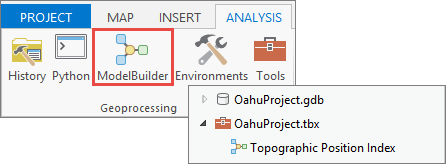
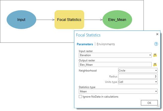
3. The Focal Statistics tool can be used to calculate the mean cell value in raster neighborhoods. Add the Focal Statistics tool to the model and fill in its parameters. Rename the Elevation bubble as Input.

   

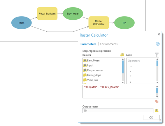
4. The Raster Calculator will be used to subtract the mean cell values from the original cell values. Add the Raster Calculator to the model and enter the following expression:"%Input%"–"%Elev_Mean%".

   

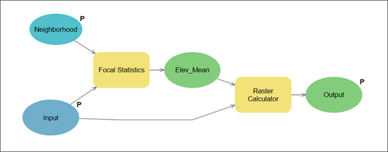
5. In order to make a stand-alone tool, some of the tool parameters should be editable. Make a variable in the Focal Statistics tool out of the Neighborhood parameter.

   

6. Make model parameters out of the Input, TPI, and Neighborhood elements by right-clicking their bubbles and checking Model Parameter. Those elements will show up as tool parameters when the tool is run. Rename TPI as Output. Save and close the model.

   

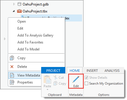
7. Now that the model is complete, the tool must be documented. Right-click your model in the Project pane and choose View Metadata. Choose Edit from the Home tab.

   

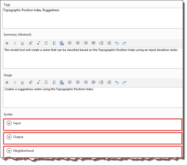
8. Create entries for the Tags, Summary, and Usage sections as well as help entries for the Input, Output, and Neighborhood parameters. Save the edits and close the editing session.

   

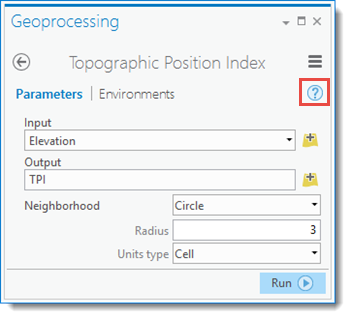
9. In the Project pane, double-click your model to open up the tool. Click the Help icon to see the help items you entered in the metadata. Click OK to run the model as a tool.

   

   Tip:

   If an error occurs when running your tool, try changing the output format to a TIFF.

10. In order to view the data correctly for the TPI the analyst must change the layer’s symbology. Open the Symbology pane and change the Symbology type to Classify. Change the method to Standard Deviation and use the Upper value to determine the standard deviation (σ) of your data. Note that the last break value may represent the highest data value and may not be useful for calculating σ. Change the Classification Method to Manual Interval and the number of Classes to 5. Leave the last break, but change the first to fourth breaks to -1σ, -0.5σ, 0.5σ and 1σ respectively. Change the Label values as seen in the dialog box below.

    

11. Turn on the Diamond Head trail layer that the analyst digitized and note the slope and TPI in the area around the trail. Move the TrailLine feature class to the top of the 2D Layers list if it is not rendering fully. The trail winds up the crater and avoids the steepest areas by using a zigzag pattern to ascend through valleys and ridges.

    

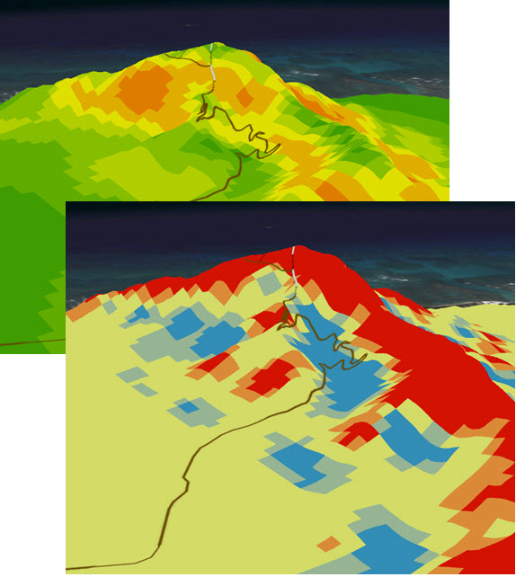
    The analyst decides that the hike will not be as difficult as choosing between Diamond Head and the Nu'uanu Pali lookout. Doing the 3D analysis was so exciting that she decides to get up early in the morning and visit both attractions.

Resources

Data Resources

Feature Class	Source
Oahu_Elevation_Contours_100ft	Hawaii Statewide GIS Program. (2014). Oahu Elevation Contours 100ft. HawaiiStateGIS. Downloaded February, 2016 from Hawaii State GIS Open Data Portal
Coastline	Hawaii Statewide GIS Program. (2014). Coastline. HawaiiStateGIS. Downloaded February, 2016 from Hawaii State GIS Open Data Portal
WorldView 2 Imagery - Oahu.tiff	Hawaii Statewide GIS Program. (2014). WorldView 2 Imagery - Oahu. HawaiiStateGIS. Downloaded February, 2016 from Hawaii State GIS Open Data Portal

Steps for digitizing the Diamond Head hiking trail using ArcGIS Pro

1. Create a new Polyline feature class by right-clicking on the destination geodatabase. For the Has Z parameter, choose No. The trail will be in 2D and draped over the elevation in the scene.

   

2. Use the Imagery Basemap as well as online maps of the Diamond Head trail to pick out points where the trail changes between walking trail, stairs, and tunnel.

   

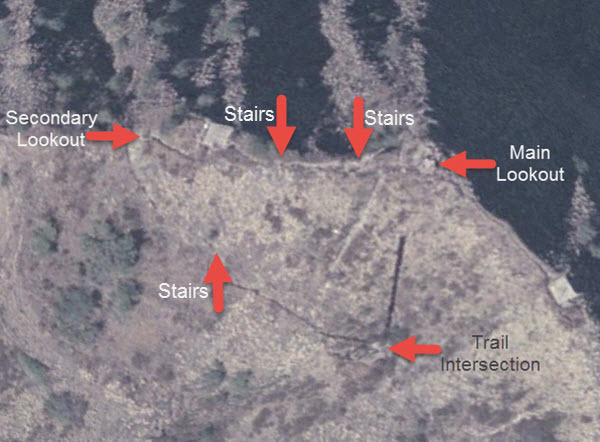
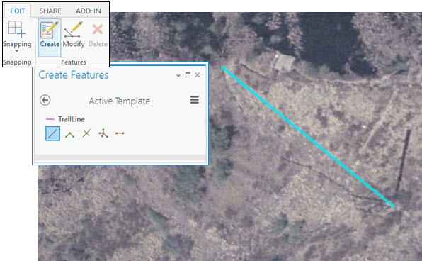
3. With the new feature class highlighted in the Contents pane, click the Create button in the Edit tab to open the Create Features pane. Make sure the Line symbol is selected in the Create Features pane. Create a line connecting the Trail Intersection and the Secondary Lookout seen above. Double-click the second point to finish drawing the line. Close the Create Features pane.

   

4. You will need to add extra vertices in order to make the line follow the actual trail. With the new feature class highlighted in the Contents pane, click the Modify button in the Edit tab to open the Modify Features pane. In the Modify pane, choose Vertices from the Reshape list and click the Add button.

   

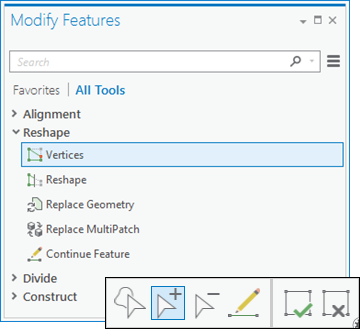
5. Click along the line to add extra vertices.

   

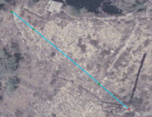
6. Use the Normal function to move the vertices to follow the trail. Save your edits.

   

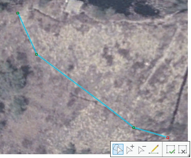
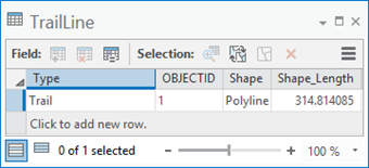
7. The hiking trail is made up of segments of trail, stairs, and tunnels. Add a new text field for the type of trail and enter Trail in the new field for the first line.

   

Note:

You cannot add a new field during an edit session. Save your edits to end the edit session before adding the new field. You will have to start a new edit session to enter a value in the new field.

8. Repeat the process for each section of the trail.

   

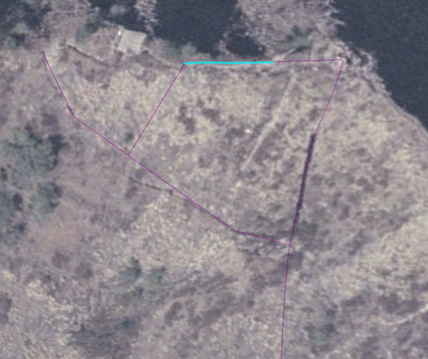
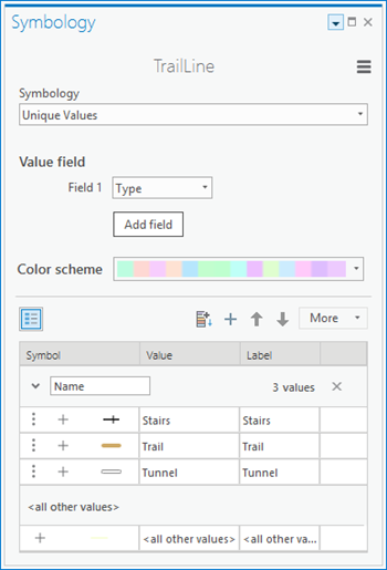
9. Use Unique Values to symbolize the trail based on the Type field.

   

References

Andrew D. Weiss. (2001). Topographic Position and Landforms Analysis. The Nature Conservancy. Accessed February 2016.

Tom Dilts. (2016). Topography Tools for ArcGIS 10.3 and earlier. University of Nevada Reno. Accessed February 2016.

Summary

This case study demonstrates a number of analytical methods that can be adapted to many different application areas, allowing you to answer a variety of questions.

Method	Generic Question	Examples
Viewshed Analysis	What is visible from specific locations?	Is the entire forest visible from the fire towers?
Creating custom tools using ModelBuilder	Should this process be automated?	Where are the hotspots for each feature class in a geodatabase? Where are the best habitats for a species in each study year?
Topographic Position Index	What is the topography of the area?	Which areas offer the most protection for wildlife? Which areas are most accessible for hikers?