Available with Spatial Analyst license.
All cost distance tools use essentially the same algorithm to calculate output. The essential difference is determined by the primary output of each tool.
Calculation of cost distance
The Cost Distance tool creates an output raster in which each cell is assigned the accumulative cost to the closest source cell. The algorithm utilizes the node/link cell representation used in graph theory. In the node/link representation, each center of a cell is considered a node and each node is connected to its adjacent nodes by multiple links.
Every link has an impedance associated with it. The impedance is derived from the costs associated with the cells at each end of the link (from the cost surface) and from the direction of movement through the cells.
The cost assigned to each cell represents the cost per unit distance for moving through the cell. The final value per cell is the cell size multiplied by the cost value. For example, if the cost raster has a cell size of 30, and a particular cell has a cost value of 10, the final cost of that cell is 300 units.
Node travel costs
The cost to travel between one node and the next is dependent on the spatial orientation of the nodes. How the cells are connected also impacts the travel cost.
Adjacent node cost
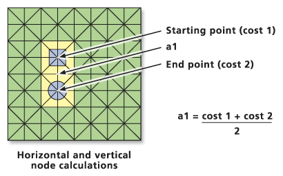
When moving from a cell to one of its four directly connected neighbors, the cost to move across the links to the neighboring node is 1 times cell 1, plus cell 2, divided by 2:
a1 = (cost1 + cost2) / 2- where:
cost1—The cost of cell 1
cost2—The cost of cell 2
a1—The total cost of the link from cell 1 to cell 2
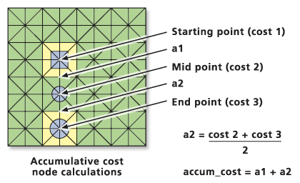
Accumulative perpendicular cost
The accumulative cost is determined by the following formula:
accum_cost = a1 + (cost2 + cost3) / 2- where:
cost2—The cost of cell 2
cost3—The cost of cell 3
a2—The cost of moving from cell 2 to 3
accum_cost—The accumulative cost to move into cell 3 from cell 1
Diagonal node cost
If the movement is diagonal, the cost to travel over the link is 1.414214 (or the square root of 2) times the cost of cell 1 plus the cost of cell 2, divided by 2:
a1 = 1.414214 (cost3 + cost2) / 2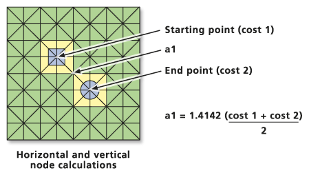
When determining the accumulative cost for diagonal movement, the following formula must be used:
accum_cost = a1 + 1.414214(cost2 + cost3) / 2Accumulative cost cell list
Creating an accumulative cost-distance raster using graph theory can be viewed as an attempt to identify the lowest-cost cell and add it to an output list. It is an iterative process that begins with the source cells. The goal of each cell is to be assigned quickly to the output cost-distance raster.
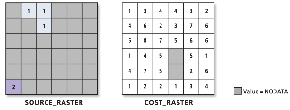
In the first iteration, the source cells are identified and assigned 0 since there is no accumulative cost to return to themselves. Next, all the source cell's neighbors are activated, and a cost is assigned to the links between the source cell nodes and the neighboring cells' nodes using the above accumulative cost formulas. Each of these neighborhood cells can reach a source; consequently, they can be chosen or assigned to the output accumulative cost raster. To be assigned to the output raster, a cell must have the next least-cost path to a source.
The accumulative cost values are arranged in a list from the lowest accumulative cost to the highest.
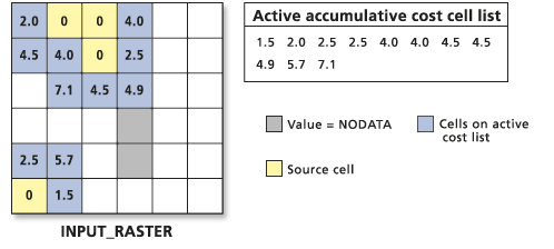
The lowest cost cell is chosen from the active accumulative cost cell list, and the value for that cell location is assigned to the output cost-distance raster. The list of active cells expands to include the neighbors of the chosen cell, because those cells now have a way to reach a source. Only those cells that can possibly reach a source can be active in the list. The cost to move into these cells is calculated using the accumulative cost formulas.
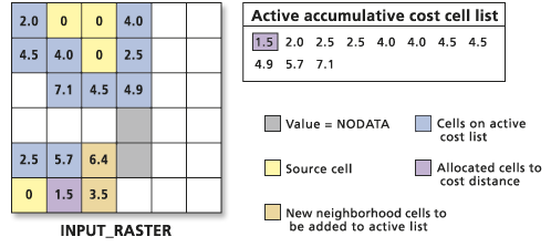
Again, the active cell on the list with the lowest cost is chosen, the neighborhood is expanded, the new costs are calculated, and the new cost cells are added to the active list.
Source cells do not have to be connected. All disconnected sources contribute equally to the active list. Only the cell with the lowest accumulative cost is chosen and expanded, regardless of the source to which it will be allocated.
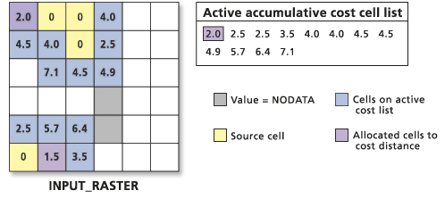
This allocation process continues. Furthermore, cells on the active list are updated if a new, cheaper route is created by the addition of new cell locations to the output raster.
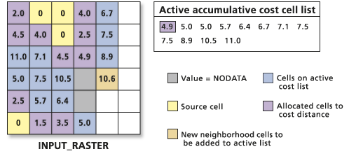
This updating can occur with the advent of new paths for cells on the active list as more cells are allocated to the output raster. When the cell with the lowest value on the active accumulative cost list is allocated to the output raster, all the accumulative costs are calculated. These costs are also calculated for the neighboring cells of the newly assigned output cell, even if the neighboring cells are on the active list through another cell. If the new accumulative cost for the locations on the active list is greater than the one the cells currently have, the value is ignored. If the accumulative cost is less, the old accumulative cost for the location is replaced on the active list with the new value. That cell, which now has access to a cheaper and more desirable path to a source, moves up the active chosen list.
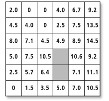
In the example below, the cell location at row 3, column 1 (highlighted by the box), had an accumulative cost of 11.0 when it was put on the active list to reach the source at the top of the raster. However, because the lower source expanded to this location, the cell had access to a cheaper accumulative cost path to reach a source. The value for the location was updated on the active list and allocated to the output earlier because of this lower accumulative cost.
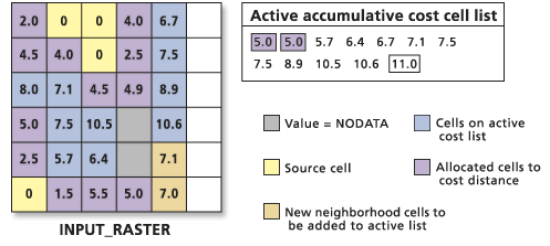
If there are multiple zones or disconnected sets of source cells on the input source raster, the growing process continues and allocates the cheapest cost cell from the active list regardless of which source it is from.
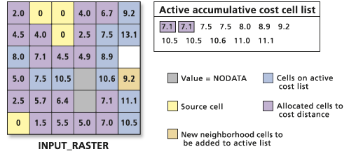
When the growth fronts meet, the least-cost path back to the source proceeds until all eligible cells have received a cost value.
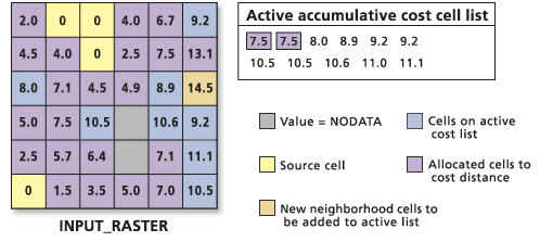
It is conceivable that when the growing patterns meet, cells from one growth pattern will be able to reach a source cell in another set or growth pattern more cheaply; if so, they will be reassigned to the new source. This behavior was shown by the cell at row 3, column 1, earlier but is also exemplified below by the cell located at row 3, column 6.
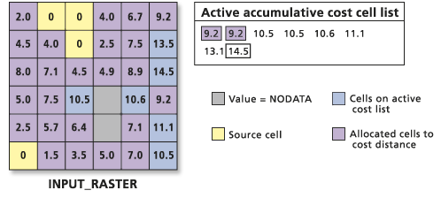
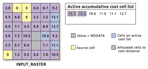
When all cells have been chosen from the active list, the result is the accumulative cost or weighted-distance raster. The procedure used ensures that the lowest accumulative cost is guaranteed for each cell. This process continues for all cells until the edge of the raster is encountered, the boundary of the window is found, or the maximum distance is reached.
No travel is allowed through cells containing NoData values. The least accumulative cost for cells on the back side of a group of NoData cells is determined by the cost to travel around these locations. If a cell location is assigned NoData on the input cost raster, NoData will be assigned to the cell location on the cost distance output raster.
