Available with Spatial Analyst license.
All path distance tools use essentially the same algorithm to calculate output. The essential difference is determined by the primary output of each tool.
The Path Distance tool is the primary tool for cost distance analysis accounting for both horizontal and vertical cost factors as well as true surface distance. The Path Distance Allocation tool employs the same algorithm but returns as its primary output a raster denoting the nearest source for each cell for each location. The Path Distance Back Link tool identifies the directionality of the neighbor that is the next cell on the least accumulative cost path to the nearest source.
Calculation of path distance
The path distance tools create an output raster in which each cell is assigned the accumulative cost from the cheapest source cell. The algorithm utilizes the node/link cell representation. In this representation, the center of a cell is considered a node, and each node is connected by links to the nodes adjacent to it.
Every link has an impedance associated with it. The impedance is derived from the costs associated with the cells at each end of the link (from the cost surface) and from the direction of movement.
To simplify the discussion, the formulas in the following section identify how travel cost is accumulated between cells over a cost surface; how to modify the cost to account for surface distance and horizontal and vertical factors will be addressed in a subsequent section.
Node travel costs
The cost to travel between one node and the next is dependent on the spatial orientation of the nodes. How the cells are connected also impacts the travel cost.
Adjacent node cost
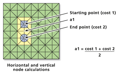
When moving from a cell to one of its four directly connected neighbors, the cost to move across the links to the neighboring node is 1 times cell 1, plus cell 2, divided by 2:
a1 = (cost1 + cost2) / 2- where:
cost1 is the cost to travel through cell 1.
cost2 is the cost to travel through cell 2.
a1 is the cost assigned to the link from cell 1 to cell 2.

Accumulative perpendicular cost
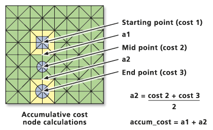
The accumulative cost is determined with the following formula:
accum_cost = a1 + (cost2 + cost3) / 2- where:
cost2 is the cost to travel through cell 2.
cost3 is the cost to travel through cell 3.
accum_cost is the accumulative cost of moving into cell 3 from cell 1.
Note: In the image below, a2 is the cost of moving from cell 2 to cell 3.

Diagonal node cost
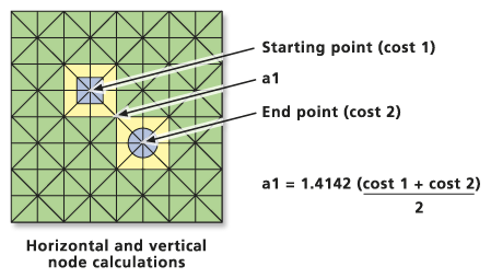
If the movement is diagonal, the cost to travel the link is 1.414214 (the square root of 2), times the cost to travel through cell 1, plus the cost to travel through cell 2, divided by 2:
a1 = 1.414214(cost1 + cost2) / 2
When determining the accumulative cost for diagonal movement, the following formula is used:
accum_cost = a1 +1.414214(cost2 + cost3) / 2Accumulative cost cell list
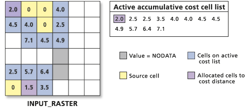
Creating an accumulative cost-distance raster using graph theory can be viewed as an attempt to identify the lowest-cost cell and add it to an output list. It is an iterative process that begins with the source cells. The goal of each cell is to be assigned quickly to the output cost-distance raster.
Comparing path distance to cost distance
The processing that occurs in path distance is similar to that of cost distance (see How the cost distance tools work). First, the source cells are identified. Then the cost to travel to each neighbor that adjoins a source cell is determined. Next, each of the neighbor cells is listed from least costly to most costly. The cell location with the least cost is removed from the list. Finally, the least accumulative cost to each of the neighbors of the cell that was removed from the list is determined.

The process is repeated until all cells on the raster have been assigned an accumulative cost. The difference between the cost distance and path distance tools is how the cost of moving from one cell to the next is computed.
Path distance formula
From the cell perspective, the objective of the path distance tools is for each cell location in the analysis extent to determine the least costly path to reach the cell from the least costly source. Each cell will need to determine the least accumulative cost path from a source, the source that allows for the least cost path, and the least cost path itself.
Path distance
The cost to move between cells over the cost surface is determined by the formulas discussed above. In Path Distance, these costs (identified as Cost_Surface in the equations below) can be modified by the surface distance (Surface_distance) and the horizontal and vertical factors. The formula used to calculate the total cost of travel from cell a to cell b depends on if that travel is perpendicular or diagonal:
- Perpendicular:
Cost_distance = (((Cost_Surface(a) * Horizontal_factor(a)) + (Cost_surface(b) * Horizontal_factor(b)))/2) * Surface_distance(ab) * Vertical_factor(ab) - Diagonal:
Cost_distance = (((Cost_Surface(a) * Horizontal_factor(a)) + (Cost_surface(b) * Horizontal_factor(b)))/2)
                * 1.414214 * Surface_distance(ab) * Vertical_factor(ab)
Note that the division by 2 of the friction of the segments is deferred until the horizontal factor is integrated.
If no cost surface is specified, then a cost of 1 per-unit distance will be used (the same as applying a cost raster with values of all 1s). Both the horizontal and vertical factors are applied to per-unit distance. Negative horizontal and vertical factors are not allowed. However, since both factors are multipliers to the accumulative cost for each cell, a factor of less than 1 but greater than 0 reduces the total cost for that cell. A vertical factor of zero, or zeros for both segments of the horizontal factors, result in a zero cost for the cell.
Accumulative cost distance
The accumulative cost to travel from cell a to cell c passing through cell b is as follows:
Accum_cost_distance = a1 + (((Cost_Surface(b) * Horizontal_factor(b)) + (Cost_surface(c)
* Horizontal_factor(c)))/2) * Surface_distance(bc) * Vertical_factor(bc)- where:
a1 is the total cost of travel from cell a to cell b.
Horizontal and vertical parameters
There are several different types of parameters you can use to control the horizontal and vertical friction factors. For each of these factors, there are various modifiers that can be used for further control over the analysis.
For more details on these parameters, proceed to the following section: