Available with 3D Analyst license.
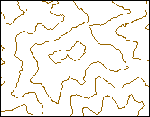
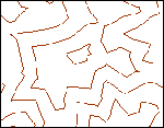
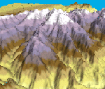
Viewing a surface in 3D offers an excellent means of understanding its shape and characteristics, as peaks, ridges and valleys can be seen in greater detail. A 2D map can also capture some of this detail through the use of contour lines, which can offer an idea about the areas with gradual and rapid slope changes. Contours offer a great means of establishing a feel for the shape of a surface, as they can be used to identify potential ridgelines and streams. In the following illustrations, the same area is displayed using a 3D hillshade of the surface and a planimetric view of its contour lines.
ArcGIS 3D Analyst extension also has tools that allow more quantitative analysis of the shape of a surface. Slope is often used in analyses to find areas with low slopes for construction or areas with high slopes, which may be prone to erosion or landslides. Aspect is often used to determine how much sun a slope will receive—for instance, to model how vegetation will grow or snow will melt or how much solar heat a building will receive.
Slope and aspect in rasters and TINs
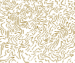
The following illustrates slope and aspect. In the picture on the left, darker shades of red indicate steeper slopes. In the picture on the right, west-facing slopes are dark blue and southeast-facing slopes are yellow.
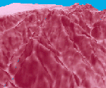
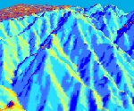
Rasters and TINs model a surface's slope and aspect in different ways. In a raster, slope and aspect are calculated for each cell by fitting a plane to the z-values of each cell and its eight surrounding neighbors. The slope or the aspect of the plane becomes the slope or aspect value of the cell in a new raster. In a triangulated irregular network (TIN), each triangle face defines a plane with a slope and an aspect. These values are quickly calculated, as needed, when you query or render the faces.
Hillshading surfaces
Hillshades indicate the distribution of light along a surface when illuminated by the light of the sun as defined by a locational bearing expressed in terms of azimuth and vertical angle. Applying a hillshade will increase the perception of depth in a 3D surface and can also be used in diverse applications that involve modeling solar insulation.
There are two ways to derive a hillshade of a surface. The first technique, which is most useful for adding depth for 3D visualization, is to turn on shading for the layer in ArcScene using the Rendering tab on the Layer Properties dialog box. This shades the layer (any surface or aerial 3D feature layer) on the fly using the scene's illumination settings. Hillshading is on by default for TINs. You must turn it on for rasters, because not all rasters are surfaces.
The following illustration demonstrates the dramatic visual impact made by the application of a hillshade:
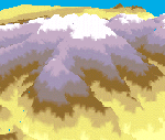

The second technique, which is useful as input for analyses and for enhancing depth in 2D surfaces in ArcMap, is to use the Hillshade Surface Analysis tool on the 3D Analyst toolbar. This creates a new hillshade raster that you can make partially transparent and display in 2D (or 3D) with an elevation layer. The following illustrates (from left to right) a 2D elevation raster, a transparent hillshade raster, and a shaded relief map.


Deriving contour lines from rasters and TINs
Contours are lines that connect all contiguous locations with the same height (or other) value in the input grid or TIN. There are two ways to create contours with ArcGIS 3D Analyst extension:
- By clicking the surface with the Contour tool
 . This creates a single contour line, which exists as a 3D graphic in a scene or map.
 - By using the Contour Surface Analysis command. This creates a series of contours with a given contour interval for the whole surface. These contours are saved as a feature class with a height attribute.
Learn more about creating contours with ArcGIS 3D Analyst extension
When you create contours from a grid, the contouring function interpolates lines between the cell centers. The lines seldom pass through the cell centers and do not follow the cell boundaries. In contrast, when you create contours from a TIN, the function interpolates straight lines across each triangle that spans the contour value using linear interpolation.
The following illustration on the left shows contours created from a raster surface. The illustration on the right shows contours created from a TIN surface.
