Summary
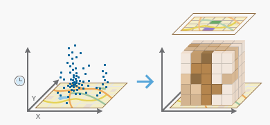
Summarizes a set of points into a netCDF data structure by aggregating them into space-time bins. Within each bin, the points are counted and specified attributes are aggregated. For all bin locations, the trend for counts and summary field values are evaluated.
Illustration

Usage
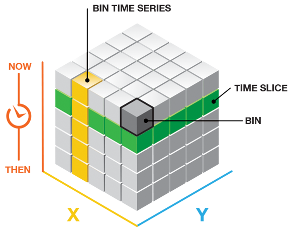
This tool aggregates your point Input Features into space-time bins. The data structure it creates may be thought of as a three-dimensional cube made up of space-time bins with the x and y dimensions representing space and the t dimension representing time.

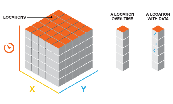
Every bin has a fixed position in space (x,y) and in time (t). Bins covering the same (x, y) area share the same location ID. Bins encompassing the same duration share the same time-step ID. Because the cube is always rectangular even if your point data is not, some locations will have point counts of zero for all time steps. For many analyses, only locations with data—with at least one point count greater than 1 for at least one time step—will be included in the analysis.

The Input Features should be points, such as crime or fire events, disease incidents, customer sales data, or traffic accidents. Each point should have a date associated with it. The field containing the event timestamp must be of type Date. The tool requires a minimum of 60 points and a variety of timestamps. The tool will fail if the parameters specified result in a cube with more than two billion bins.
This tool requires projected data to accurately measure distances.
Output from this tool is a netCDF representation of your input points as well as messages summarizing cube characteristics written to the Results window. The netCDF file created may be used as input to the Emerging Hot Spot Analysis tool. See Visualizing the Space Time Cube to get strategies allowing you to look at cube contents.
Select a field of type Date for the Time Field parameter. This field should contain the timestamp associated with each point feature.
The Time Step Interval defines how you want to partition your aggregated points across time. You might decide to aggregate points using one-day, one-week, or one-year intervals, for example. Time-step intervals are always fixed durations, and the tool requires a minimum of ten time steps. If you do not provide a Time Step Interval value, the tool will calculate one for you. See Learn more about how the Create Space Time Cube tool works for details on how default time-step intervals are computed. Valid time-step interval units are Years, Months, Days, Hours, Minutes, and Seconds.
Type the Time Step Interval as an integer value and a unit value. Example time-step interval entries are 1 Weeks, 2 Weeks, 13 Days, or 1 Months.
If your space-time cube cannot be created, the tool may be unable to structure the data you have provided into ten time-step intervals. If you get an error message running this tool, examine the timestamps of the input points to make sure they include a range of values. The range of values must span at least ten seconds as this is the smallest time increment that the tool will take. Ten time-step intervals are required by the Mann-Kendall statistic.
When creating a space time cube with incident data, depending on the Time Step Interval that you choose, it is possible to create a bin at the beginning or end of the cube that does not have data across the entire span of time. For instance, if you choose a 1 month Time Step Interval, and your data does not break up evenly into 1 month intervals, then there will be a time step at either the beginning or end that does not have data over its entire span. This can bias your results because it will appear that the temporally biased time step has significantly less points than other time steps, which is in fact an artificial result of the aggregation scheme. The messages indicate whether there is temporal bias in the first or last time step. One solution is to create a selection set of your data so that it does fall evenly within the desired Time Step Interval.
It is not uncommon for a dataset to have a regularly spaced temporal distribution. For instance, you might have yearly data that all falls on January 1st of each year, or monthly data that is all timestamped the first of each month. This kind of data is often referred to as panel data. With panel data, temporal bias calculations will often show very high percentages. This is to be expected, as each bin will only cover one particular time unit in the given time step. For instance, if you chose a 1 Year Time Step Interval and your data fell on January 1st of each year, then each bin would only cover one day out of the year. This is perfectly acceptable since it applies to each bin. Temporal bias becomes an issue when it is only present for certain bins due to bin creation parameters rather than true data distribution. It is important to evaluate the temporal bias in terms of the expected coverage in each bin based on your data's distribution.
The temporal bias in the output report is calculated as the percentage of the time span that has no data present. For example, an empty bin would have 100% temporal bias. A bin with a 1 month time span and an end Time Step Alignment that only has data for the second two weeks of the first time step would have a 50% first time step temporal bias. A bin with a 1 month time span and a start Time Step Alignment that only has data for the first two weeks of the last time step would have a 50% last time step temporal bias.
Once you create a space-time cube, the spatial extent of the cube can never be extended. If further analysis of the space-time cube will involve the use of a study area (such as a Polygon Analysis Mask in the Emerging Hot Spot Analysis tool) you will want to ensure that the Polygon Analysis Mask does not extend beyond the extent of the Input Features when you create your cube. Setting the study area polygon(s) that you will use in future analysis as the Extent environment setting when you create the cube will ensure that the extent of the cube is as large as you need it to be at the beginning of your analysis.
You can create a Template Cube that can be used each time you run your analysis, especially if you want to compare data for a series of time periods. By providing the same template cube, you ensure the extent of your analysis, bin size, time-step interval, reference time, and time-step alignment are always consistent.
If you provide a Template Cube, input points that fall outside of the template cube extent will be excluded from analysis. Also, if the spatial reference associated with the input point features is different from the spatial reference associated with the template cube, the tool will project the Input Features to match the template cube before beginning the aggregation process. The spatial reference associated with the template cube will override Output Coordinate System settings as well. In addition, the Template Cube, when specified, will determine the processing extent used, even if you specify a different processing extent. See How Create Space Time Cube works for more information.
The Reference Time may be a date and time value or just a date value; it may not be just a time value. The expected format is determined by the computer's regional time settings.
The Distance Interval specifies how large the space-time bins should be. The bins are used to aggregate your point data. You may decide to make each bin 50 meters by 50 meters, for example. Unless a Template Cube is specified, the bin in the upper left corner of the cube will be centered on the upper left corner of the spatial extent for your Input Features. You will want to select a distance interval that makes sense to your analysis. You should find the balance between making your distance interval too large and losing the underlying patterns in your point data, and making your distance interval too small so you end up with a cube filled with zero counts. If you do not provide a Distance Interval value, the tool will calculate one for you. See How Create Space Time Cube works for details on how default distance intervals are computed. The distance interval units supported are Kilometers, Meters, Miles, and Feet.
The trend analysis performed on the aggregated count data and summary field values is based on the Mann-Kendall statistic.
The following statistical operations are available for the aggregation of attributes with this tool: Sum, Mean, Minimum, Maximum, Standard Deviation, and Median.
When filling empty bins with SPATIAL_NEIGHBORS, a Queens Case Contiguity is used (contiguity based on edges and corners) of the 2nd order (includes neighbors and neighbors of neighbors). A minimum of 4 spatial neighbors are required to fill the empty bin using this option.
When filling empty bins with SPACE_TIME_NEIGHBORS, a Queens Case Contiguity is used (contiguity based on edges and corners) of the 2nd order (includes neighbors and neighbors of neighbors). Additionally, temporal neighbors are used for each of those bins found to be spatial neighbors by going backward and forward 2 time steps. A minimum of 13 space time neighbors are required to fill the empty bin using this option.
When filling empty bins with a temporal trend TEMPORAL_TREND, the first two time periods and last two time periods at a given location must have values in their bins in order to interpolate values at other time periods for that location.
The TEMPORAL_TREND fill type uses the Interpolated Univariate Spline method in SciPy's Interpolation package.
Null values present in any of the summary field records will result in those features being excluded from analysis. If having the count of points in each bin is part of your analysis strategy, you may want to consider creating separate cubes, one for the count (without Summary Fields) and one for Summary Fields. If the set of null values is different for each summary field, you may also consider creating a separate cube for each summary field.
Syntax
CreateSpaceTimeCube(in_features, output_cube, time_field, {template_cube}, {time_step_interval}, {time_step_alignment}, {reference_time}, {distance_interval}, summary_fields)| Parameter | Explanation | Data Type |
in_features | The input point feature class to be aggregated into space-time bins. | Feature Layer |
output_cube | The output netCDF data cube that will be created to contain counts and summaries of the input feature point data. | File |
time_field |
The field containing the date and time (timestamp) for each point. This field must be of type Date. | Field |
template_cube (Optional) | A reference space-time cube used to define the output_cube extent of analysis, bin dimensions, and bin alignment. The time_step_interval, distance_interval, and reference_time values are also obtained from the template cube. This template cube must be a netCDF (.nc) file that has been created using this tool. | File |
time_step_interval (Optional) | The number of seconds, minutes, hours, days, weeks, or years that will represent a single time step. All points within the same Time Step Interval and Distance Interval will be aggregated. (When a Template Cube is provided, this parameter is ignored, and the Time Step Interval value is obtained from the template cube). Examples of valid entries for this parameter are 1 Weeks, 13 Days, or 1 Years. | Time unit |
time_step_alignment (Optional) | Defines how aggregation will occur based on a given time_step_interval. If a template_cube is provided, the time_step_alignment associated with the template_cube overrides this parameter setting and the time_step_alignment of the template_cube is used.
| String |
reference_time (Optional) | The date/time to use to align the time-step intervals. If you want to bin your data weekly from Monday to Sunday, for example, you could set a reference time of Sunday at midnight to ensure bins break between Sunday and Monday at midnight. (When a template_cube is provided, this parameter is ignored and the reference_time is based on the template_cube.) | Date |
distance_interval (Optional) | The spatial extent of the bins used to aggregate the in_features. All points that fall within the same distance_interval and time_step_interval will be aggregated. (When a template_cube is provided, this parameter is ignored and the distance interval value will be based on the template_cube.) | Linear unit |
summary_fields | The numeric field containing attribute values used to calculate the specified statistic when aggregating into a space-time cube. Multiple statistic and field combinations may be specified. Null values are excluded from all statistical calculations. Available statistic types are:
Available fill types are:
Note: Null values present in any of the summary fields will result in those features being excluded from analysis. If having the count of points in each bin is part of your analysis strategy, you may want to consider creating separate cubes, one for the count (without summary fields) and one for summary fields. If the set of null values is different for each summary field, you may also consider creating a separate cube for each summary field. | Value Table |
Code sample
CreateSpaceTimeCube example 1 (Python window)
The following Python window script demonstrates how to use the CreateSpaceTimeCube tool.
arcpy.env.workspace = r"C:\STPM"
arcpy.CreateSpaceTimeCube_stpm("Homicides.shp", "Homicides.nc", "OccDate", "#", "3 Months",
                               "End time", "#", "3 Miles", "Property MEDIAN SPACETIME; Age STD ZEROS")
CreateSpaceTimeCube example 2 (stand-alone Python script)
The following stand-alone Python script demonstrates how to use the CreateSpaceTimeCube tool.
# Create Space Time Cube of homicide incidents in a metropolitan area

# Import system modules
import arcpy

# Set geoprocessor object property to overwrite existing output, by default
arcpy.env.overwriteOutput = True

# Local variables...
workspace = r"C:\STPM"

try:
    # Set the current workspace (to avoid having to specify the full path to the feature
    # classes each time)
    arcpy.env.workspace = workspace

    # Create Space Time Cube of homicide incident data with 3 months and 3 miles settings
				# Also aggregate the median of property loss, no date predicted by space-time neighbors
				#	Also aggregate the standard deviation of the victim's age, fill the no-data with zeros
    # Process: Create Space Time Cube
    cube = arcpy.CreateSpaceTimeCube_stpm("Homicides.shp", "Homicides.nc", "MyDate", "#",
                                          "3 Months", "End time", "#", "3 Miles", "Property MEDIAN SPACETIME; Age STD ZEROS")

    # Create a polygon that defines where incidents are possible
    # Process: Minimum Bounding Geometry of homicide incident data
    arcpy.MinimumBoundingGeometry_management("Homicides.shp", "bounding.shp", "CONVEX_HULL",
                                             "ALL", "#", "NO_MBG_FIELDS")

    # Emerging Hot Spot Analysis of homicide incident cube using 5 Miles neighborhood
    # distance and 2 neighborhood time step to detect hot spots
    # Process: Emerging Hot Spot Analysis
    cube = arcpy.EmergingHotSpotAnalysis_stpm("Homicides.nc", "COUNT", "EHS_Homicides.shp",
                                              "5 Miles", 2, "bounding.shp")

except arcpy.ExecuteError:
    # If any error occurred when running the tool, print the messages
    print(arcpy.GetMessages())
Environments
Licensing information
- ArcGIS Desktop Basic: Yes
- ArcGIS Desktop Standard: Yes
- ArcGIS Desktop Advanced: Yes