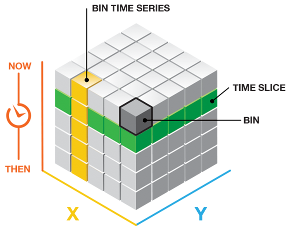
The Create Space Time Cube tool takes timestamped point features and structures them into a netCDF data cube by aggregating the points into space-time bins. Within each bin the points are counted, any Summary Field statistics are calculated, and the trend for bin values across time at each location is measured using the Mann-Kendall statistic. You would most likely use this tool to create the input cube needed for further space-time pattern mining, but you could also use it to examine time-series trends across your study area.
Interpreting results
Output from this tool is a netCDF representation of your input points. You may visualize the cube point count data in either 2D or 3D using ArcGIS Pro. In addition to the netCDF file, messages summarizing the space-time cube dimensions and contents are written to the Results window. Right-clicking on the Messages entry in the Results window and selecting View will display the results in a Message dialog box.
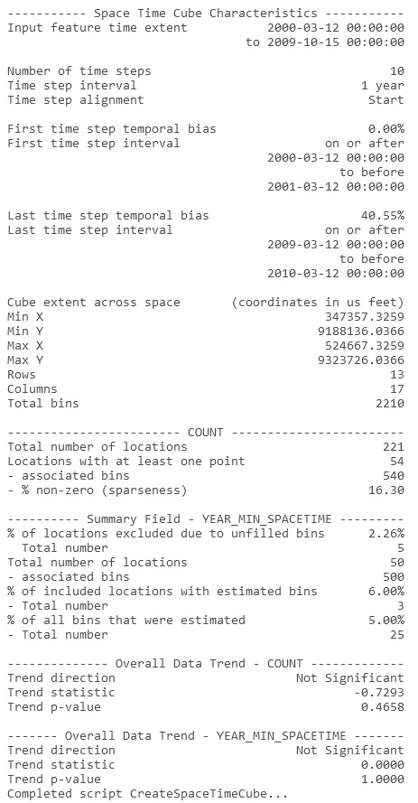
The cube structure will have rows, columns, and time steps. If you multiply the number of rows by the number of columns by the number of time steps, you will obtain the total number of bins in the cube. The rows and columns determine the spatial extent of the cube, while the time steps determine the temporal extent.
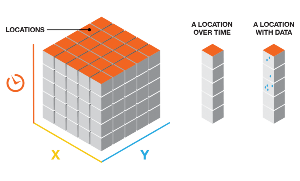
For most analyses, only locations with data for at least one time-step interval will be included in the analysis, but they will be analyzed across all time steps. When computing point counts, zero counts are assumed for any bin where there are no points, but the associated location has had at least one point for at least one time-step interval. Information about the percentage of zeros associated with locations that have data for a least one time-step interval is reported in the messages as sparseness. When computing values for Summary Fields, the Fill Empty Bins with parameter determines how bins with no points will be filled. Any bins that cannot be filled based on the estimation criteria will result in the whole location being excluded from the analysis. A minimum of 4 neighbors are required to fill empty bins using the average value of spatial neighbors and a minimum of 13 neighbors are required to fill empty bins using the average value of space time neighbors.
At the end of the output message there is information about the Overall Data Trend. This trend is based on an aspatial time-series analysis. The question it answers is, overall, are the events represented by the input points increasing or decreasing over time? To obtain the answer, the number of points for all locations in each time-step interval is analyzed as a time series of count values using the Mann-Kendall statistic.
Bin dimensions for aggregation
In most cases you will know how to define the cube bin dimensions, and the strong recommendation is that you think about what the appropriate dimensions should be for the particular questions you are trying to answer. If you are looking at crime events, for example, you may decide to aggregate points into 400-meter or 0.25-mile bins because that is your city block size. If you have data covering an entire year, you might decide to look at trends in terms of monthly or weekly event aggregation.
Default parameters
In the rare case where you do not have strong justification for any particular time-step interval or distance interval, you can leave the Time Step Interval or Distance Interval parameter blank and let the tool calculate default values for you.
The default bin distance is calculated as follows:
- Determine the distance of the longest side of the Input Features extent (maximum extent).
- The bin distance is then the larger of either the maximum extent divided by 100 or an algorithm based on the spatial distribution of the Input Features.
The default time-step interval is based on two different algorithms used to determine the optimal number and width of time-step intervals. The minimum numeric result from these algorithms, larger than ten, is used for the default number of time-step intervals. When both numeric results are less than ten, ten becomes the default number of time-step intervals.
Time Step Alignment
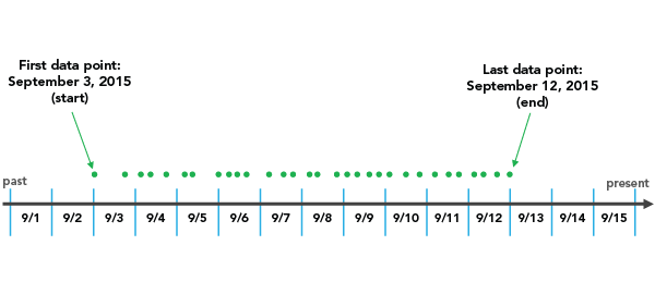
The Time Step Alignment is an important parameter to think about when aggregating your data into a space-time cube, because it determines where the aggregation will begin and end. Let's take a look at an example.
End time
If an END_TIME Time Step Alignment is chosen with a Time Step Interval of 3 days, for instance, the binning will initiate with the last data point and go back in 3 day increments until all data points fall within a time step.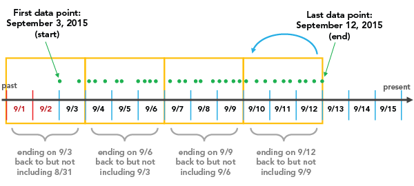
It is important to note that, depending on the Time Step Interval that you choose, it is possible to create a time step at the beginning of the space-time cube that does not have data across the entire span of time. In the example above, you'll notice that 9/1 and 9/2 are included in the first time step even though no data exists until 9/3. These empty days are part of the time step, but have no data associated with them. This can bias your results because it will appear that the temporally biased time step has significantly less points than other time steps, which is in fact an artificial result of the aggregation scheme. The report indicates whether there is temporal bias in the first or last time step. In this case, 2 out of the 3 days in the first time step have no data, so the temporal bias would be 66%.
END_TIME is the default option for Time Step Alignment because many analyses are focused on what has happened most recently, so putting this bias towards the beginning of the cube is preferable. Another solution, which gets rid of the temporal bias all together, would be to provide data that is divided evenly by the Time Step Interval so that no time periods are biased. You can do this by creating a selection set of the data that excludes the part of the point dataset that falls outside of what you would like to be the first time period. In this example, selecting all data except for those that fall before 9/4 would solve the problem. The report shows the time span of the first and last time steps, and that information can be used to determine where to make the cutoff.
It is also important to note that if, in the process of moving back in time, the final bin happened to land exactly on the first data point as its start, that final data point would not be included in that bin. This is because with an END_TIME Time Step Alignment each bin includes the last date in a given bin, yet goes back to but does not include the first date in that bin. So, in this case an additional bin would have to be added to ensure that the first data point was included.
Start time
If a START_TIME Time Step Alignment is chosen, with a Time Step Interval of 3 days, for instance, then binning will start at the first data point and go in 3 day increments until the last data point falls within the final time step.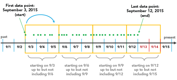
There are a few things that are important to note. One is that with a START_TIME Time Step Alignment, based on the Time Step Interval that you choose, it is possible to create a time step at the end of the space-time cube that does not have data across the entire span of time. In the example above, you'll notice that 9/13 and 9/14 are included in the last time step even though no data exists after 9/12. These empty days are part of the time step, but have no data associated with them. This can bias your results because it will appear that the temporally biased time step has significantly less points than other time steps, which is in fact an artificial result of the aggregation scheme. The report indicates whether there is temporal bias in the first or last time step. In this case, 2 out of the 3 days in the last time step have no data, so the temporal bias would be 66%. This is particularly problematic when choosing a START_TIME Time Step Alignment because analyses that are focused on the most recent data can be significantly impacted. The solution would be to provide data that is divided evenly by the Time Step Interval so that no time periods are biased. You can do this by creating a selection set of the data and that excludes the part of the point dataset that falls outside of what you would like to be the last time period. In this example, selecting all data except for those that fall after 9/11 would solve the problem. You could also choose to cut 2 days from the beginning of the dataset, which would also lead to the data falling evenly within the time steps. The report shows the time span of the first and last time steps, and that information can be used to determine where to make the cutoff.
It is also important to note that if, in the process of moving forward in time, the final time step happened to land exactly on the last data point as its end, that final data point would not be included in that bin. This is because with a START_TIME Time Step Alignment each bin includes the first date in a given bin, yet goes forward to but does not include the last date in that bin. So, in this case an additional bin would have to be added to ensure that the last data point was included.
Reference Time
A REFERENCE_TIME Time Step Alignment allows you to ensure that a specific date marks the beginning or end of one of the time steps in the cube.
When you choose a REFERENCE_TIME that falls
after the extent of the dataset, at the last data point, or in the
middle of the dataset, it will be treated as the last data point of
a time step and all other bins on either side will be created using
an Time Step Alignment until all of the data is covered,
as illustrated below.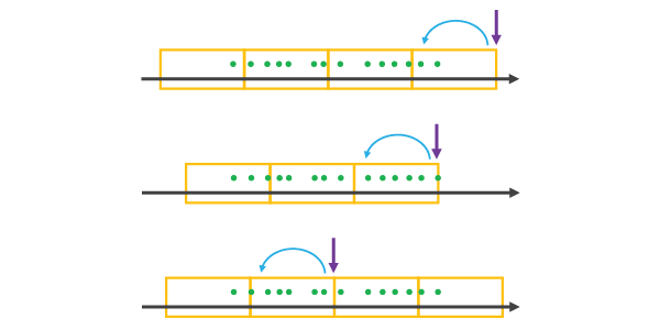
When you choose a REFERENCE_TIME that falls before the extent of the dataset or at the first data point, it will be treated as the first data point of a time step and all other time steps on either side will be created using a START_TIME Time Step Alignment until all of the data is covered, as illustrated below.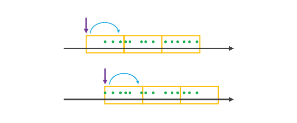
Note that choosing a REFERENCE_TIME before or after the extent of your data has the potential to create empty or partially empty bins, which can bias your analysis.
Template Cubes
Choosing to use a Template Cube allows you to use a consistent spatial extent and Time Step Interval while analyzing different datasets. For example, you might use last year's space-time cube as a Template Cube once the next year's data is acquired, as this will ensure consistency in both the spatial extent and the Time Step Interval being used, while allowing the cube to extend to cover the new data. You might also use the space time cube for one type of incident as the Template Cube for analyzing another type of incident, to ensure that a comparison of analysis results is valid.
Choosing a Template Cube has implications for
the Time Step Alignment. Let's take a look at a few examples. When you
choose a Template Cube that falls before or after the time span of
the Input Features, time steps will be added until all of the data
is covered by a time step, using the Time Step Alignment of the
Template Cube. The resulting space-time cube will have empty cubes
wherever the Template Cube did not overlap the Input Features in
time. This can bias the results of analysis. If the Template Cubeoverlaps the Input Features, the resulting space-time cube will
cover the temporal extent of the Template Cube and extend until all Input Features are covered, using the Time Step Alignment of the
Template Cube. The illustration below shows Template Cubes in blue,
and the resulting space-time cubes in orange.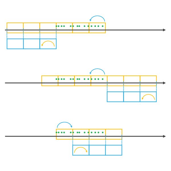
It is important to note that when creating a new space-time cube using a Template Cube, the temporal extent of the Template Cube will be extended until all data is covered. This will allow you to use last year's cube to create a new cube that includes both last year's data and this year's data. The spatial extent of the Template Cube is treated differently. Any data falling outside of the spatial extent of the Template Cube will be dropped from the analysis. The Template Cube and the resulting space-time cube will have identical spatial extents. The only changes that can occur are within the spatial extent where locations that previously had no data can become locations with data if new features have appeared that were not present when the Template Cube was created.
Trend analysis
The Mann-Kendall trend test is performed on every location with data as an independent bin time-series test. The Mann-Kendall statistic is a rank correlation analysis for the bin count or value and their time sequence. The bin value for the first time period is compared to the bin value for the second. If the first is smaller than the second, the result is a +1. If the first is larger than the second, the result is -1. If the two values are tied, the result is zero. The result for each pair of time periods compared are summed. The expected sum is zero, indicating no trend in the values over time. Based on the variance for the values in the bin time series, the number of ties, and the number of time periods, the observed sum is compared to the expected sum (zero) to determine if the difference is statistically significant or not. The trend for each bin time series is recorded as a z-score and a p-value. A small p-value indicates the trend is statistically significant. The sign associated with the z-score determines if the trend is an increase in bin values (positive z-score) or a decrease in bin values (negative z-score). Strategies for visualizing the trend results are provided in Visualizing the Space Time Cube.
Additional resources
Histogram bin-width optimization
- Shimazaki H. and Shinomoto S., A method for selecting the bin size of a time histogram in Neural Computation (2007) Vol. 19(6), 1503–1527.
- Online Statistics Education: A Multimedia Course of Study (http://onlinestatbook.com/). Project leader: David M. Lane, Rice University (chapter 2, "Graphing Distributions, Histograms").
Mann-Kendall trend test
- Hamed, K. H., Exact distribution of the Mann-Kendall trend test statistic for persistent data in Journal of Hydrology (2009), 86–94.
- Kendall, M. G., Gibbons, J. D., Rank correlation methods, fifth ed., (1990) Griffin, London.
- Mann, H. B., Nonparametric tests against trend in Econometrica (1945) Vol. 13, 245–259.