Proximity analysis

One of the most basic questions asked of a GIS is "what's near what?" For example:

• How close is this well to a landfill?
• Do any roads pass within 1,000 meters of a stream?
• What is the distance between two locations?
• What is the nearest or farthest feature from something?
• What is the distance between each feature in a layer and the features in another layer?
• What is the shortest street network route from some location to another?

Proximity tools can be divided into two categories depending on the type of input the tool accepts: features or rasters. The feature-based tools vary in the types of output they produce. For example, the Buffer tool outputs polygon features, which can then be used as input to overlay or spatial selection tools such as Select Layer By Location. The Near tool adds a distance measurement attribute to the input features. The raster-based Euclidean distance tools measure distances from the center of source cells to the center of destination cells. The raster-based cost-distance tools accumulate the cost of each cell traversed between sources and destinations.

Feature-based proximity tools

For feature data, the tools found in the Proximity toolset can be used to discover proximity relationships. These tools output information with buffer features or tables. Buffers are usually used to delineate protected zones around features or to show areas of influence. For example, you might buffer a school by one mile and use the buffer to select all the students that live more than one mile from the school to plan for their transportation to and from school. You could use the multiring buffer tool to classify the areas around a feature into near, moderate distance, and long distance classes for an analysis. Buffers are sometimes used to clip data to a given study area or to exclude features within a critical distance of something from further consideration in an analysis.

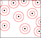
Buffer and Multiple Ring Buffer create area features at a specified distance (or several specified distances) around the input features.

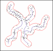
Below are examples of buffered lines and points:

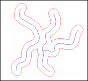
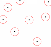
Below is an example of multiple ring buffers:

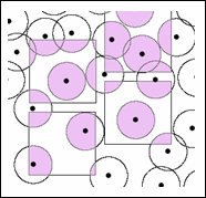
Buffers can be used to select features in another feature class, or they can be combined with other features using an overlay tool, to find parts of features that fall in the buffer areas.

Below is an example of buffered points overlaid with polygon features:

Below is an example of a study area clipped to a buffer area:

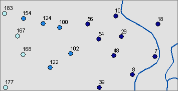
The Near tool calculates the distance from each point in one feature class to the nearest point or line feature in another feature class. You might use Near to find the closest stream for a set of wildlife observations or the closest bus stops to a set of tourist destinations. The Near tool will also add the Feature Identifier and, optionally, coordinates of and the angle toward the nearest feature.

Below is an example showing points near river features. The points are symbolized using graduated colors based on distance to a river, and they're labeled with the distance.

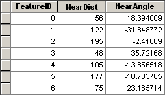
Below is part of the attribute table of the points, showing the distance to the nearest river feature:

Point Distance calculates the distance from each point in one feature class to all the points within a given search radius in another feature class. This table can be used for statistical analyses, or it can be joined to one of the feature classes to show the distance to points in the other feature class.

You can use the Point Distance tool to look at proximity relationships between two sets of things. For example, you might compare the distances between one set of points representing several types of businesses (such as theaters, fast food restaurants, engineering firms, and hardware stores) and another set of points representing the locations of community problems (litter, broken windows, spray-paint graffiti), limiting the search to one mile to look for local relationships. You could join the resulting table to the business and problem attribute tables and calculate summary statistics for the distances between types of business and problems. You might find a stronger correlation for some pairs than for others and use your results to target the placement of public trash cans or police patrols.

You might also use Point Distance to find the distance and direction to all the water wells within a given distance of a test well where you identified a contaminant.

Below is an example of point distance analysis. Each point in one feature class is given the ID, distance, and direction to the nearest point in another feature class.

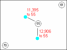
Below is the Point Distance table, joined to one set of points and used to select the points that are closest to point 55.

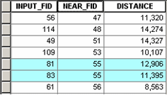
Both Near and Point Distance return the distance information as numeric attributes in the input point feature attribute table for Near and in a stand-alone table that contains the Feature IDs of the Input and Near features for Point Distance.

Create Thiessen Polygons creates polygon features that divide the available space and allocate it to the nearest point feature. The result is similar to the Euclidean Allocation tool for rasters. Thiessen polygons are sometimes used instead of interpolation to generalize a set of sample measurements to the areas closest to them. Thiessen polygons are sometimes also known as Proximal polygons. They can be thought of as modeling the catchment area for the points, as the area inside any given polygon is closer to that polygon's point than any other.

Below is an example of Thiessen polygons for a set of points.

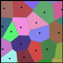
You might use Thiessen polygons to generalize measurements from a set of climate instruments to the areas around them or to quickly model the service areas for a set of stores.

Layer and Table View tools

Select Layer By Location allows you to change the set of selected features in ArcMap by finding features in one layer that are within a given distance of (or share one of several other spatial relationships with) features in another feature class or layer. Unlike the other vector tools, Select By Location does not create new features or attributes. The Select Layer By Location tool is in the Layers and Table Views toolset, or you can Select By Location from the ArcMap Selection menu.

Below is an example where points within a given distance of other points are selected—the buffers are shown only to illustrate the distance.

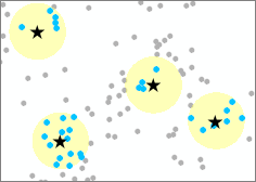
You could use Select By Location to find all the highways within a county or all the houses within five kilometers of a wildfire.

Network distance tools

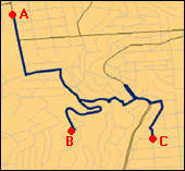
Some distance analyses require that the measurements be constrained to a road, stream, or other linear network. ArcGIS Network Analyst lets you find the shortest route to a location along a network of transportation routes, find the closest point to a given point, or build service areas (areas that are equally distant from a point along all available paths) in a transportation network.

Below is an example of a Route solution for three points along a road network. The Closest Facility solution will find locations on the network that are closest (in terms of route distance) to an origin.

Below is an example of a Service Area of travel time on a network:

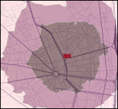
Network Analyst keeps a running total of the length of the segments as it compares various alternative routes between locations when finding the shortest route. When finding service areas, Network Analyst explores out to a maximum distance along each of the available network segments, and the ends of these paths become points on the perimeter of the service area polygon.

Network Analyst can also compute Origin-Destination matrices, which are tables of distances between one set of points (the Origins) and another set of points (the Destinations).

Raster-based distance tools

The ArcGIS Spatial Analyst extension provides several sets of tools that can be used in proximity analysis. The Distance toolset contains tools that create rasters showing the distance of each cell from a set of features or that allocate each cell to the closest feature. Distance tools can also calculate the shortest path across a surface or the corridor between two locations that minimizes two sets of costs. Distance surfaces are often used as inputs for overlay analyses; for example, in a model of habitat suitability, distance from streams could be an important factor for water-loving species, or distance from roads could be a factor for timid species.

Euclidean distance

Euclidean distance is straight-line distance, or distance measured "as the crow flies." For a given set of input features, the minimum distance to a feature is calculated for every cell.

Below is an example of the output of the Euclidean Distance tool, where each cell of the output raster has the distance to the nearest river feature:

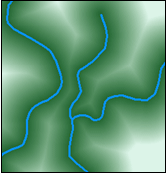
You might use Euclidean Distance as part of a forest fire model, where the probability of a given cell igniting is a function of distance from a currently burning cell.

Euclidean allocation

Euclidean allocation divides an area up and allocates each cell to the nearest input feature. This is analogous to creating Thiessen polygons with vector data. The Euclidean Allocation tool creates polygonal raster zones that show the locations that are closest to a given point. If you specify a maximum distance for the allocation, the results are analogous to buffering the source features.

Below is an example of a Euclidean allocation analysis where each cell of the output raster is given the ID of the nearest point feature:

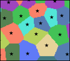
You might use Euclidean allocation to model zones of influence or resource catchments for a set of settlements.

Below is an example of a Euclidean allocation analysis where each cell within a specified distance of a point is given the ID of the nearest point feature:

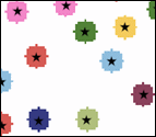
For each cell, the color indicates the value of the nearest point; in the second graphic, a maximum distance limits the allocation to buffer-like areas. You might use Euclidean allocation with a maximum distance to create a set of buffer zones around streams.

Euclidean direction

Euclidean direction gives each cell a value that indicates the direction of the nearest input feature.

Below is an example of the output of the Euclidean Direction tool where each cell of the output raster has the direction to the nearest point feature:

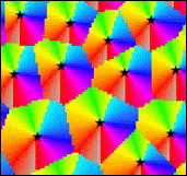
You might use Euclidean direction to answer the question, For any given cell, which way do I go to get to the nearest store?

Cost distance

In contrast with the Euclidean distance tools, cost distance tools take into account that distance can also be measured in cost (for example, energy expenditure, difficulty, or hazard) and that travel cost can vary with terrain, ground cover, or other factors.

Given a set of points, you could divide the area between them with the Euclidean allocation tools so that each zone of the output would contain all the areas closest to a given point. However, if the cost to travel between the points varied according to some characteristic of the area between them, then a given location might be closer, in terms of travel cost, to a different point.

Below is an example of using the Cost Allocation tool, where travel cost increases with land-cover type. The dark areas could represent difficult-to-traverse swamps, and the light areas could represent more easily traversed grassland.

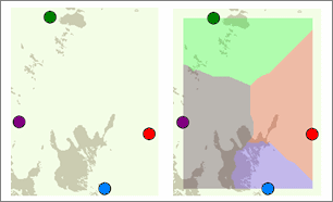
Compare the Euclidean allocation results with the Cost allocation results.

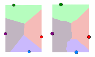
This is in some respects a more complicated way of dealing with distance than using straight lines, but it is very useful for modeling movement across a surface that is not uniform.

Path distance

The path distance tools extend the cost distance tools, allowing you to use a cost raster but also take into account the additional distance traveled when moving over hills, the cost of moving up or down various slopes, and an additional horizontal cost factor in the analysis.

For example, two locations in a long, narrow mountain valley might be further apart than one is from a similar location in the next valley over, but the total cost to traverse the terrain might be much lower within the valley than across the mountains. Various factors could contribute to this total cost, for example:

• It is more difficult to move through brush on the mountainside than through meadows in the valley.
• It is more difficult to move against the wind on the mountain side than to move with the wind and easier still to move without wind in the valley.
• The path over the mountain is longer than the linear distance between the endpoints of the path, because of the additional up and down travel.
• A path that follows a contour or cuts obliquely across a steep slope might be less difficult than a path directly up or down the slope.

The path distance tools allow you to model such complex problems by breaking travel costs into several components that can be specified separately. These include a cost raster (such as you would use with the Cost tools), an elevation raster that is used to calculate the surface-length of travel, an optional horizontal factor raster (such as wind direction), and an optional vertical factor raster (such as an elevation raster). In addition, you can control how the costs of the horizontal and vertical factors are affected by the direction of travel with respect to the factor raster.

Below is an example of the Path Distance Allocation tool, where several factors contribute to cost.

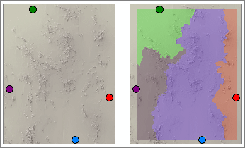
The illustration below compares the Euclidean Allocation results with the Path Distance Allocation analysis:

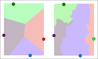
The Corridor tool finds the cells between locations that minimize travel cost using two different cost distance surfaces. For example, you might use the tool to identify areas that an animal might cross while moving from one part of a park to another.

Below are examples of two sets of factors that might affect the cost of traveling across a landscape. In this case, one is land-cover type, and the other is slope.

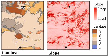
For each of the factors, the Cost Distance tool can be used to find the travel cost from one or more locations.

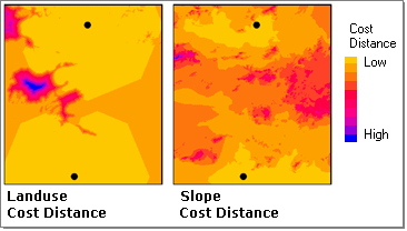
The Corridor tool combines the results of the Cost Distance analysis for the two factors. The results can be reclassified to find the areas where the combined costs are kept below a certain level. These areas might be more attractive corridors for the animal to travel within.

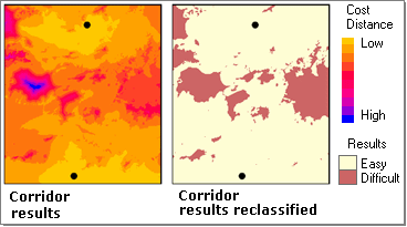
The Surface length tool in the ArcGIS 3D Analyst toolbox in the Functional Surface toolset calculates the length of input line features given a terrain surface. This length can be significantly longer than the two-dimensional, or planimetric, length of a feature in hilly or mountainous terrain. Just as a curving path between two points is longer than a straight path, a path that traverses hills and valleys is longer than a perfectly level path. The surface length information is added to the attribute table of the input line features.

Below is an example that contrasts the surface length of a line feature in rough terrain with its planimetric length.

Proximity tools

Vector distance tools

Tool	Location	What it does
Buffer	Analysis toolbox/Proximity toolset	Creates new feature data with feature boundaries at a specified distance from input features
Near	Analysis toolbox/Proximity toolset	Adds attribute fields to a point feature class containing distance, feature identifier, angle, and coordinates of the nearest point or line feature
Select By Location	Data Management toolbox/Layers and Table Views toolset	Selects features from a target feature class within a given distance of (or using other spatial relationships) the input features
Create Thiessen Polygons	Analysis toolbox/Proximity toolset	Creates polygons of the areas closest to each feature for a set of input features
Make Closest Facility Layer	Network Analyst/Analysis toolset	Sets analysis parameters to find the closest location or set of locations on a network to another location or set of locations
Make Service Area Layer	Network Analyst/Analysis toolset	Sets analysis parameters to find polygons that define the area within a given distance along a network in all directions from one or more locations
Make Route Layer	Network Analyst/Analysis toolset	Sets analysis parameters to find the shortest path among a set of points
Make OD Cost Matrix Layer	Network Analyst/Analysis toolset	Sets analysis parameters to create a matrix of network distances among two sets of points

Table of vector distance tools with location and description

Raster distance tools

Raster distance tools are located in ArcToolbox in the Distance toolset (in the Spatial Analyst Tools toolbox) and the Functional Surface toolset (in the 3D Analyst Tools toolbox).

Tool	Location	What it does
Euclidean Distance	Spatial Analyst/Distance toolset	Calculates the distance to the nearest source for each cell.
Euclidean Allocation	Spatial Analyst/Distance toolset	Gives each cell the identifier of the closest source.
Euclidean Direction	Spatial Analyst/Distance toolset	Calculates the direction to the nearest source for each cell.
Cost Distance	Spatial Analyst/Distance toolset	Calculates the distance to the nearest source for each cell, minimizing cost specified in a cost surface.
Cost Allocation	Spatial Analyst/Distance toolset	Gives each cell the identifier of the closest source, minimizing cost specified in a cost surface.
Cost Path	Spatial Analyst/Distance toolset	Calculates the least-cost path from a source to a destination, minimizing cost specified in a cost surface.
Cost Back Link	Spatial Analyst/Distance toolset	Identifies for each cell the neighboring cell that is on the least-cost path from a source to a destination, minimizing cost specified in a cost surface.
Path Distance	Spatial Analyst/Distance toolset	Calculates the distance to the nearest source for each cell, minimizing horizontal cost specified in a cost surface, as well as the terrain-based costs of surface distance and vertical travel difficulty specified by a terrain raster and vertical cost parameters.
Path Distance Allocation	Spatial Analyst/Distance toolset	Gives each cell the identifier of the closest source, minimizing horizontal cost specified in a cost surface, as well as the terrain-based costs of surface distance and vertical travel difficulty specified by a terrain raster and vertical cost parameters.
Path Distance Back Link	Spatial Analyst/Distance toolset	Identifies for each cell the neighboring cell that is on the least-cost path from a source to a destination, minimizing horizontal cost specified in a cost surface, as well as the terrain-based costs of surface distance and vertical travel difficulty specified by a terrain raster and vertical cost parameters.
Corridor	Spatial Analyst/Distance toolset	Calculates the sum of accumulative cost for two input cost distance rasters. The cells below a given threshold value define an area, or corridor, between sources where the two costs are minimized.
Surface Length	3D Analyst/Functional Surface toolset	Calculates the length of line features across a surface, accounting for terrain.

Table of raster distance tools with location and description